【MATLAB项目实战】基于Morlet小波变换的滚动轴承故障特征提取研究

轴承在运行过程中发生点蚀、剥落、擦伤等表面损伤类故障时,在损伤部位产生的突变冲击脉冲力作用下,会形成周期性冲击振动。而小波变换具有良好的时频分辨率和瞬态检测能力,非常适合处理此类非平稳信号。根据小波变换原理,小波变换系数对应信号局部与各小波基函数的相似程度,即系数值越大,相似程度越高,鉴于Morlet小波形状与上述轴承故障信号的冲击特征相似,利用连续小波变换对信号进行细致的时间尺度网格刻划,可以在轴承表面损伤早期提取振动信号中的冲击特征。以上小波变换过程可以理解为一种滤波行为，相关研究也是通过优化 Morlet小波参数和尺度参数,实现 Morlet小波与信号的较好匹配,获得最佳滤波效果。对信号滤波后可以有效检测轴承故障早期的冲击特征。

附件中Signal.mat为一段监测轴承状态的加速度传感器信号。轴承的结构参数和运行参数信息如表1所示。故障类型（正常、内圈故障、外圈故障、滚动体故障和保持架故障）。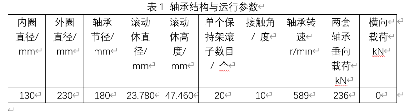

以内圈故障为例：

以外圈故障为例：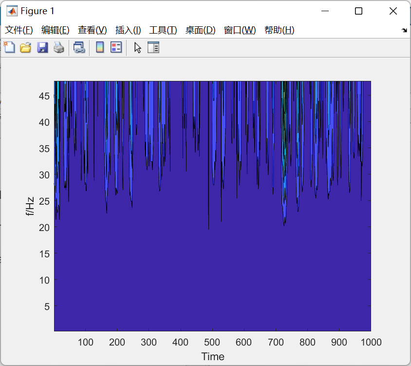

clc;
clear;
load O-A-1.mat
channel_1=Channel_1(1:1000,:);
fs=100;
[y,f,coi] = cwt(channel_1,fs);
figure
contourf(1:1:1000,f,abs(y))
xlabel('Time')
ylabel('f/Hz')

function [y,f,coi] = cwt(x,fs,varargin)
%-INPUT--------------------------------------------------------------------
% x: input signal (must be real vector for now)
% fs: sampling frequency in Hz
% varargins: pair of parameter name and value
%   'wavetype': 'morse'(default) or 'morlet'
%   'g': morse gamma parameter (default=3)
%   'b': morse beta parameter (default=20)
%   'k': order of morse waves (default=0)
%   's0': smallest scale (determined automatically by default)
%   'no': number of octaves (determined automatically by default)
%   'nv': number of voices per octave (default=10)
%   'pad': whether to pad input signal (default=true)
%-OUTPUT-------------------------------------------------------------------
% y: output time-frequency spectrum (complex matrix)
% f: frequency bins (in Hz) of spectrum
% coi: edge of cone of influence (in Hz) at each time point
%==========================================================================
% Author: Colin M McCrimmon
% E-mail: [email protected].edu
%==========================================================================

params.wavetype = 'morlet';
params.g = 3;
params.b = 20;
params.k = 0;
params.s0 = [];
params.no = [];
params.nv = 10;
params.pad = true;
for i = 1:2:numel(varargin)
    params.(varargin{
    i}) = varargin{
    i+1};
end
params.b = max(params.b,ceil(3/params.g)); % >=3
params.b = min(params.b,fix(120/params.g)); % <= 120
params.nv = 2*ceil(params.nv/2); % even;
params.nv = max(params.nv,4); % >=4
params.nv = min(params.nv,48); % <= 48

x = x(:);
x = x(end:-1:1);
x = detrend(x,0);
norig = numel(x);

npad = 0;
if params.pad
    npad = floor(norig/2);
    x =[conj(x(npad:-1:1)); x; conj(x(end:-1:end-npad+1))];
end
n = numel(x);

[s,~,params.no] = getScales(params.wavetype,norig,params.s0,params.no,params.nv,params.g,params.b);
w = getOmega(n);

switch params.wavetype
    case 'morse'
        wc = getMorseCenterFreq(params.g,params.b);
        psihat = morse(s,w,wc,params.g,params.b,params.k);
        f = wc ./ (2 * pi * s);
        [~,sigma] = getMorseSigma(params.g,params.b);
        coival = 2 * pi / (sigma * wc);
    case 'morlet'
        wc = 6;
        psihat = morlet(s,w,wc);
        f = wc ./ (2 * pi * s);
        sigma = 1 / sqrt(2);
        coival = 2 * pi / (sigma * wc);
end

xhat = fft(x);
y = ifft((xhat * ones(1,size(psihat,2))) .* psihat);
y = y(1+npad:norig+npad,:).';

f = fs * f.';

coi = 1 ./ (coival*(1/fs)*[1E-5,1:((norig+1)/2-1),fliplr((1:(norig/2-1))),1E-5]).';
coi(coi>max(f)) = max(f);

if nargout<1
    t = linspace(0,(size(y,2)-1)/fs,size(y,2));
    plotspectrum(t,f,y,coi);
end

end


function [scales,s0,no] = getScales(wavetype,n,s0,no,nv,g,b)
    switch wavetype
        case 'morse'
            %smallest scale
            if ~exist('s0','var') || isempty(s0)
                a = 1;
                testomegas = linspace(0,12*pi,1001);
                omega = testomegas(find( log(testomegas.^b) + (-testomegas.^g) - log(a/2) + (b/g)*(1+(log(g)-log(b))) > 0, 1, 'last'));
                s0 = min(2,omega/pi);
            end
            [~,sigma] = getMorseSigma(g,b);
        case 'morlet'
            %smallest scale
            if ~exist('s0','var') || isempty(s0)
                a = 0.1; omega0 = 6;
                omega = sqrt(-2*log(a)) + omega0;
                s0 = min(2,omega/pi);
            end
            sigma = sqrt(2)/2;
    end
    %largest scale
    hi = floor(n/(2*sigma*s0));
    if hi <=  1, hi = floor(n/2); end
    hi = floor(nv * log2(hi));    
    if exist('no','var') && ~isempty(no)
        hi = min(nv*no,hi);
    else
        no = hi/nv;
    end
    octaves = (1/nv) * (0:hi);
    scales = s0 * 2 .^ octaves;
end


function omega = getOmega(n)
	% Frequency vector sampling the Fourier transform of the wavelet
    omega = (2*pi/n) * (1:fix(n/2));
    omega = [0, omega, -omega(fix((n-1)/2):-1:1)].';
end


function wc = getMorseCenterFreq(g,b)
%Center frequency (in radians/sec) of morse wavelet with parameters gamma=g and beta=b
if b~=0
    wc = exp((1/g)*(log(b)-log(g)));
else
    wc = log(2)^(1/g);
end
end


function [sigmafreq,sigmatime] = getMorseSigma(g,b)
a = (2/g) * (log(g) - log(2*b));
sigmafreq = real(sqrt(exp(a + gammaln((2*b+3)/g) - gammaln((2*b+1)/g)) - exp(a + 2*gammaln((2*b+2)/g) - 2*gammaln((2*b+1)/g))));

c1 = (2/g)*log(2*b/g) + 2*log(b) + gammaln((2*(b-1)+1)/g) - gammaln((2*b+1)/g);
c2 = ((2-2*g)/g)*log(2) + (2/g)*log(b/g) + 2*log(g) + gammaln((2*(b-1+g)+1)/g) - gammaln((2*b+1)/g);
c3 = ((2-g)/g)*log(2) + (1+2/g)*log(b) + (1-2/g)*log(g) + log(2) + gammaln((2*(b-1+g./2)+1)/g) - gammaln((2*b+1)/g);
sigmatime = real(sqrt(exp(c1) + exp(c2) - exp(c3)));
end

function plotspectrum(t,f,y,coi)
%-INPUT--------------------------------------------------------------------
% t: time (in seconds) of the spectrum and original signal
% f: frequency bins (in Hz) of the spectrum
% y: output time-frequency spectrum (complex matrix)
% coi: edge of cone of influence (in Hz) at each time point
%-OUTPUT-------------------------------------------------------------------
% none: creates new figure and plots the time-frequency spectrum

[t,coiweightt,ut] = engunits(t,'unicode','time');
xlbl = ['Time (',ut,')'];
[f,coiweightf,uf] = engunits(f,'unicode');
%coiweightf = 1; uf = ''; %6/24/2018
ylbl = ['Frequency (',uf,'Hz)'];
coi = coi * coiweightt * coiweightf;

hf = figure;
hf.NextPlot = 'replace';
ax = axes('parent',hf);
imagesc(ax,t,log2(f),abs(y));

cmap = jet(1000);cmap = cmap([round(linspace(1,375,250)),376:875],:); %jet is convention, but let's adjust
%cmap = parula(750);
colormap(cmap)

logyticks = round(log2(min(f))):round(log2(max(f)));
ax.YLim = log2([min(f), max(f)]);
ax.YTick = logyticks;
ax.YDir = 'normal';
set(ax,'YLim',log2([min(f),max(f)]), ...
    'layer','top', ...
    'YTick',logyticks(:), ...
    'YTickLabel',num2str(sprintf('%g\n',2.^logyticks)), ...
    'layer','top')
title('Magnitude Scalogram');
xlabel(xlbl);
ylabel(ylbl);
hcol = colorbar;
hcol.Label.String = 'Magnitude';
hold(ax,'on');

%shade out complement of coi
plot(ax,t,log2(coi),'w--','linewidth',2);
A1 = area(ax,t,log2(coi),min([min(ax.YLim) min(coi)]));
A1.EdgeColor = 'none';
A1.FaceColor = [0.5 0.5 0.5];
alpha(A1,0.8);
hold(ax,'off');
hf.NextPlot = 'replace';
    
end

function [psihat,psi] = morse(s,w,wpk,g,b,k)
%-INPUT--------------------------------------------------------------------
% s: scales used (related to frequency of generated morse wave)
% w: frequencies for conducting analysis in FFT order starting with 0 (size equals number of points in frequency/time domain)
% wc: center frequency for morse wavelet (related to g and b below)
% g: gamma - use 3 for Airy wavelets
% b: beta - increase for high frequency precision but low temporal precision
% k: order of wavelets - typically only need k = 0
%-OUTPUT-------------------------------------------------------------------
% psihat: morse wavelet in frequency domain
% psi: morse wavelet in time domain
%==========================================================================
% Adapted from SC Olhede and AT Walden in "Generalized Morse
% Wavelets", 2002 IEEE TSP and Lilly, J. M. (2015), jLab: A data analysis
% package for Matlab
%
% Author: Colin M McCrimmon
% E-mail: [email protected].edu
%==========================================================================

nw = numel(w);
ns = numel(s);
s = s(:).';
w = w(:);

r = (2*b+1)/g;
c = r - 1;
i = 1:(fix(nw/2)+1);
WS = w(i) * s;
if b~=0
    a = 2 * sqrt(exp(gammaln(r) + gammaln(k+1) - gammaln(k+r))) * exp(-b*log(wpk) + wpk^g + b*log(WS) - WS.^g);
else
    a = 2 * exp(-WS.^g);
end
a(1,:) = (1/2) * a(1,:);
a(isnan(a)) = 0;

psihat = zeros(nw,ns);
psihat(i,:) = a .* laguerre(2*WS.^g,k,c);
psihat(isinf(psihat)) = 0;

psihat = psihat .* (complex(exp(1i * pi * linspace(0,nw-1,nw).')) * ones(1,ns));
psihat(2:end,s<0) = psihat(end:-1:2,s<0); %conj in time domain = conj reversal in freq domain
psihat(:,s<0) = conj(psihat(:,s<0));

if nargout>1
    psi = ifft(psihat);
end

end


function Y = laguerre(X,k,c)
% compute generalized Laguerre poly L_k^c(x) - much faster than laguerreL
Y = zeros(size(X));
sn = -1;
for m=0:k
    sn = -sn;
    Y = Y + sn * exp(gammaln(k+c+1) - gammaln(k-m+1) - gammaln(c+m+1) - gammaln(m+1)) * X.^m;
end
end

function [ psihat, psi ] = morlet(s,w,wc)
%-INPUT--------------------------------------------------------------------
% s: scales used (related to frequency of generated morse wave)
% w: frequencies for conducting analysis in FFT order starting with 0 (size equals number of points in frequency/time domain)
% wc: center frequency for morlet wavelet (usually set to 6)
%-OUTPUT-------------------------------------------------------------------
% psihat: morlet wavelet in frequency domain
% psi: morlet wavelet in time domain
%==========================================================================
% Author: Colin M McCrimmon
% E-mail: [email protected].edu
%==========================================================================

nw = numel(w);
ns = numel(s);
s = s(:).';
w = w(:);

% psihat = 2 * (exp(-(1/2)*(abs(w)*s - wc).^2) - exp(-(1/2)*wc^2));
psihat = (exp(1i*2*pi*wc*s-s.^2/10))/sqrt(pi*10);
% psihat = psihat .* (complex(exp(1i * pi * linspace(0,nw-1,nw).')) * ones(1,ns));
psihat(2:end,s<0) = psihat(end:-1:2,s<0); %conj in time domain = conj reversal in freq domain
psihat(:,s<0) = conj(psihat(:,s<0));

if nargout>1
    psi = ifft(psihat);
end

end

代码（包括数据和word）：https://download.csdn.net/download/qq_45047246/86339256