当前位置:网站首页>Tensorflow Experiment 4 -- Boston house price forecast
Tensorflow Experiment 4 -- Boston house price forecast
2022-04-22 09:41:00 【Alone.】
Boston house price forecast
The Boston house price data set includes 506 Samples , Each sample includes 12 Two characteristic variables and the average house price in the region ( The unit price ) Obviously, it is related to multiple characteristic variables , Not univariate linear regression ( Univariate linear regression ) The problem selects multiple characteristic variables to establish a linear equation , This is multivariable linear regression ( Multiple linear regression ) Problem Boston house price forecast
Data set interpretation 、
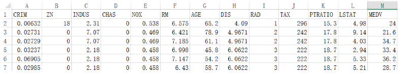
CRIM: Crime rate per capita in cities and towns
ZN: More than 25000 sq.ft. The proportion of
INDUS: The proportion of Urban Non retail commercial land
CHAS: The boundary is the river 1, otherwise 0
NOX: Nitric oxide concentration
RM: Interpretation of residential average room data set
AGE: 1940 Proportion of self use houses built before
DIS: To Boston 5 The weighted distance between two central regions
RAD: Proximity index of radial highway
TAX : Every time 10000 The full value property tax rate of US dollars
PTRATIO: The proportion of teachers and students in the city
LSTAT: The proportion of the population in the lower ranks
MEDV: The average price of a house , Company : Thousand dollars
Reading data
import tensorflow.compat.v1 as tf
import numpy as np
import matplotlib.pyplot as plt
%matplotlib inline
import pandas as pd
from sklearn.utils import shuffle
from sklearn.preprocessing import scale
print("Tensorflow The version is :",tf.__version__)

adopt Pandas Import data
df = pd.read_csv("E:/wps/boston.csv",header=0)  # The path here is the absolute path where you store the Boston house price file
print(df.describe())

Pandas Reading data
Display the first three data
df.head(3)

Display the last three pieces of data
df.tail(3)

Data set partitioning
Data preparation
ds = df.values
print(ds.shape)
print(ds)

Divide feature data and label data
x_data = ds[:,:12]
y_data = ds[:,12]
print('x_data shape=',x_data.shape)
print('y_data shape=',y_data.shape)

Divide the training set 、 Validation set and test set
train_num = 300
valid_num = 100
test_num = len(x_data) - train_num -valid_num

x_train =x_data[:train_num]
y_train =y_data[:train_num]

x_valid = x_data[train_num:train_num+valid_num]
y_valid = y_data[train_num:train_num+valid_num]

x_test = x_data[train_num+valid_num:train_num+valid_num+test_num]
y_test = y_data[train_num+valid_num:train_num+valid_num+test_num]
Convert data type
x_train = tf.cast(scale(x_train),dtype=tf.float32)
x_valid = tf.cast(scale(x_valid),dtype=tf.float32)
x_test = tf.cast(scale(x_test),dtype=tf.float32)
Notice that there is a situation , Here we use a scale() function , If this function is not applicable, the training result will be abnormal , The following picture will appear ,train_loss and valid_loss It's not worth it

Build the model
Defining models
The multiple linear regression model is still a simple linear function , Its basic form is still 𝑦=𝑤∗𝑥+𝑏, Just here 𝑤 and 𝑏 No longer a scalar , The shape will be different . According to the model definition , It performs matrix cross multiplication , So what I call here is tf.matmul() function .
def model(x,w,b):
    return tf.matmul(x,w) + b
Create variables to be optimized
W = tf.Variable(tf.random.normal([12,1],mean=0.0,stddev=1.0,dtype=tf.float32))
B = tf.Variable(tf.zeros(1),dtype = tf.float32)
print(W)
print(B)

model training
Set super parameters
This column will use the small batch gradient descent algorithm MBGD To optimize
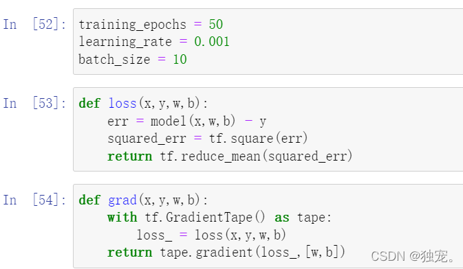
training_epochs = 50
learning_rate = 0.001
batch_size = 10
Set up a batch_size Hyperparameters , Used to adjust the number of samples optimized for small batch training each time
Define the mean square loss function
def loss(x,y,w,b):
    err = model(x,w,b) - y
    squared_err = tf.square(err)
    return tf.reduce_mean(squared_err)
Define the gradient calculation function
def grad(x,y,w,b):
    with tf.GradientTape() as tape:
        loss_ = loss(x,y,w,b)
    return tape.gradient(loss_,[w,b])
Choose the optimizer
optimizer = tf.keras.optimizers.SGD(learning_rate)
Use tf.keras.optimizers.SGD() A gradient descent optimizer is declared (Optimizer), Its learning rate is specified by parameters . The optimizer can help update the model parameters according to the calculated derivation results , Thus minimizing the loss function , The specific use method is to call its apply_gradients() Method .
Iterative training
loss_list_train = []
loss_list_valid = []
total_step = int(train_num/batch_size)

for epoch in range(training_epochs):
    for step in range(total_step):
        xs = x_train[step*batch_size:(step+1)*batch_size,:]
        ys = y_train[step*batch_size:(step+1)*batch_size]

        grads = grad(xs,ys,W,B)
        optimizer.apply_gradients(zip(grads,[W,B]))

    loss_train = loss(x_train,y_train,W,B).numpy()
    loss_valid = loss(x_valid,y_valid,W,B).numpy()
    loss_list_train.append(loss_train)
    loss_list_valid.append(loss_valid)
    print("epoch={:3d},train_loss{:.4f},valid_loss{:.4f}".format(epoch+1,loss_train,loss_valid)

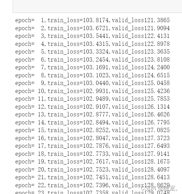
This operation train_loss and valid_loss You have all the values
Visualization loss value
plt.xlabel("Epochs")
plt.ylabel("Loss")
plt.plot(loss_list_train,'blue',label="Train Loss")
plt.plot(loss_list_valid,'red',label='Valid Loss')
plt.legend(loc=1)

Note here that the more times you execute , The greater the loss value , The greater the distance between the two lines , For example, below

View the loss of the test set
print("Test_loss:{:.4f}".format(loss(x_test,y_test,W,B).numpy()))
Choose one at random from the test set
test_house_id = np.random.randint(0,test_num)
y = y_test[test_house_id]
y_pred = model(x_test,W,B)[test_house_id]
y_predit=tf.reshape(y_pred,()).numpy()
print("House id",test_house_id,"Actual value",y,"Predicted value",y_predit)

That's it !!!
版权声明
本文为[Alone.]所创,转载请带上原文链接,感谢
https://yzsam.com/2022/04/202204220932045825.html
边栏推荐
- Analysis of the factors affecting the switching speed of MOS transistor Kia MOS transistor
- L3-002 special stack (30 points) (two points stack)
- L3-007 天梯地图 (30 分)(条件dij
- LC301. 删除无效的括号
- L2-033 simple calculator (25 points)
- Does pytorch model load the running test set and the running test set in the training process have inconsistent results?
- Design example of large range continuous adjustable (0 ~ 45V) low power stabilized voltage power supply based on MOSFET control
- 杰理之通常影响CPU性能测试结果的因素有:【篇】
- How to calculate the maximum switching frequency of MOS tube - Kia MOS tube
- L3-005 dustbin distribution (30 points) (dijkstar)
猜你喜欢

Softing dataFEED OPC Suite:赋予工业设备物联网连接能力

GS waveform analysis of depth resolved MOS transistor Kia MOS transistor

Development of esp-01s in Arduino (1)

2022年熔化焊接与热切割操作证考试题模拟考试平台操作

软件测试基础知识,看完就可以和面试官硬碰硬

【C语言进阶10——字符和字符串函数及其模拟实现(1)】
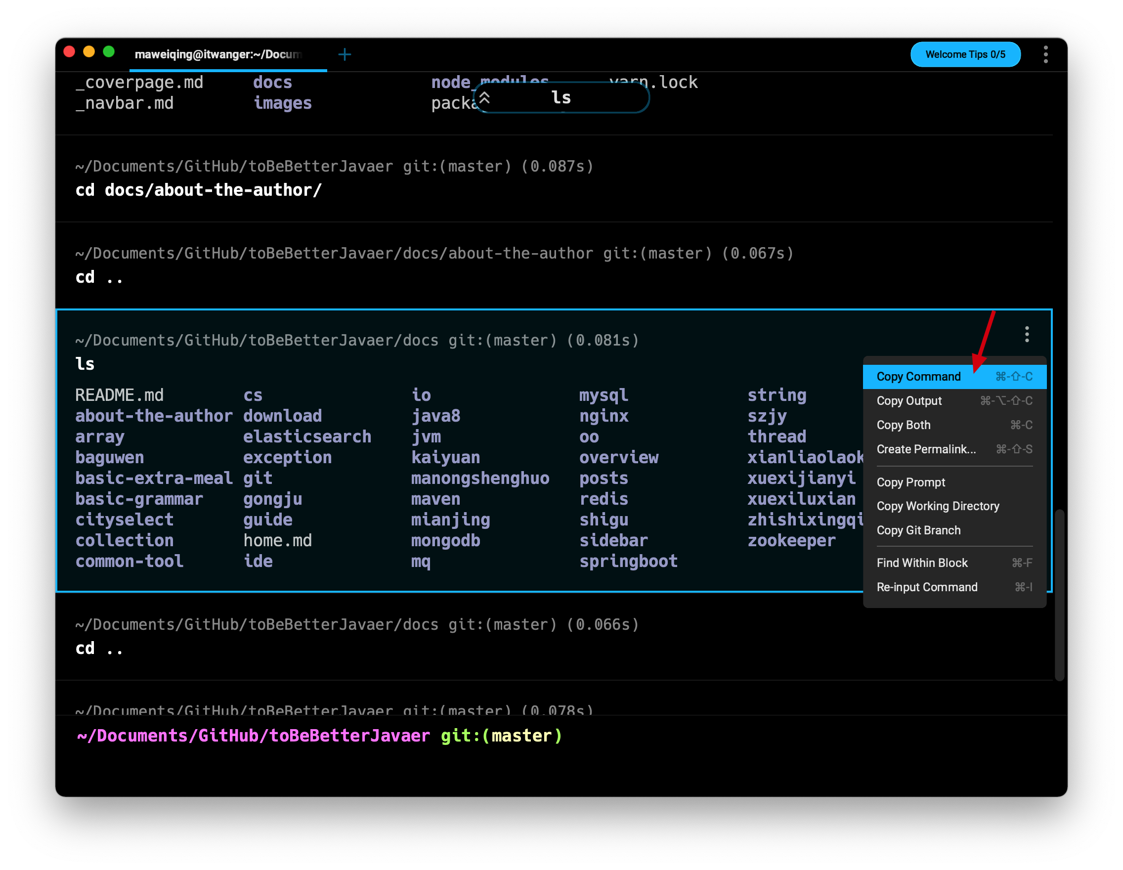
超越 iTerm!号称下一代 Terminal 终端神器,用完爱不释手!

WEB应用扫码获取浙政钉用户信息
Quantitative investment learning -- Introduction to orderflow

Aardio - 【库】webp图片转换
随机推荐
MOS管驱动电路及注意事项-KIA MOS管
How to select Bi tools? These three questions are the key
Matplotlib tutorial 04 --- drawing commonly used graphics
SQL 操作符
[SQL Server] SQL overview
超越iTerm! 号称下一代终端神器,功能贼强大!
2022-04-21 mysql-innodb存储引擎核心处理
云原生爱好者周刊:寻找 Netlify 开源替代品
L2-032 彩虹瓶 (25 分)(栈
加密压缩备份BAT脚本
Deep learning remote sensing scene classification data set sorting
Review of QT layout management
matplotlib教程04---绘制常用的图形
LC301. Remove invalid parentheses
获取浏览器网址 地址
Da14580ble light LED
Command ‘yum‘ not found, but can be installed with: apt install yum
项目实训-读报僵尸
杰理之AI Server【篇】
js老生常谈之this,constructor ,prototype