logisticRetour au chapitre

L'ensemble de données correspond à l'ensemble de données de la section précédente,Cette analyse est divisée en fonction de la question de savoir si l'utilisateur est un utilisateur très réactif,UtiliserlogisticLa régression prédit la réactivité de l'utilisateur,Probabilité d'obtenir une réponse.Régression linéaire,Voir le chapitre précédent

1 Lire et prévisualiser les données

Charger la lecture des données,Les données sont toujours désensibilisées,

file_path<-"data_response_model.csv" #change the location

# read in data
options(stringsAsFactors = F)
raw<-read.csv(file_path)   #read in your csv data
str(raw)     #check the varibale type
View(raw)    #take a quick look at the data
summary(raw) #take a quick look at the summary of variable

# response variable
View(table(raw$dv_response))  #Y
View(prop.table(table(raw$dv_response))) #Y frequency

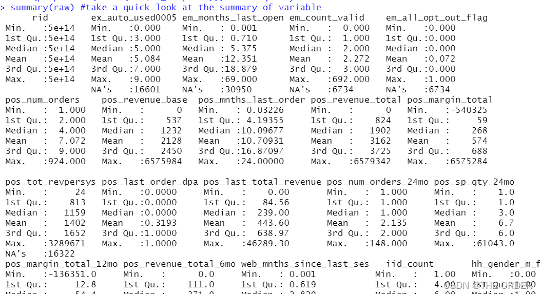
Sur la base de l'entreprise ,Les donnéesy La valeur est le taux de réponse est dv_response, Et observer son état

2 Division des données

Toujours diviser les données en trois parties ,Ensemble de formation,Ensembles de vérification et d'essai.

#Separate Build Sample
train<-raw[raw$segment=='build',]  #select build sample, it should be random selected when you build the model
View(table(train$segment))         #check segment
View(table(train$dv_response))     #check Y distribution  
View(prop.table(table(train$dv_response))) #check Y distribution

#Separate invalidation Sample
test<-raw[raw$segment=='inval',] #select invalidation(OOS) sample
View(table(test$segment))       #check segment
View(prop.table(table(test$dv_response))) #check Y distribution

#Separate out of validation Sample
validation<-raw[raw$segment=='outval',] #select out of validation(OOT) sample
View(table(validation$segment)) #check segment
View(prop.table(table(validation$dv_response))) #check Y distribution

3 profilngProduction

Additionner les taux de réponse dans les données , Les clients très réactifs dans les données originales sont: 1, Les clients à faible réponse sont 0. Le total est le nombre de clients très réactifs ,length C'est le nombre total d'enregistrements , La moyenne est la moyenne globale

# overall performance
overall_cnt=nrow(train)   #calculate the total count
overall_resp=sum(train$dv_response)  #calculate the total responders count
overall_resp_rate=overall_resp/overall_cnt  #calculate the response rate
overall_perf<-c(overall_count=overall_cnt,overall_responders=overall_resp,overall_response_rate=overall_resp_rate) #combine
overall_perf<-c(overall_cnt=nrow(train),overall_resp=sum(train$dv_response),overall_resp_rate=sum(train$dv_response)/nrow(train)) #combine
View(t(overall_perf))  #take a look at the summary

La Division ici est comme celle du chapitre précédent. lift Production graphique ,Également disponiblesqlÉcrivez la Déclaration,Commegroup by, Calculer le taux de réponse moyen par groupe par rapport au taux de réponse global .
InlibraryAvant,Télécharger d'abordplyrSac,Écris.sqlÀ téléchargersqldf
install.packages(“sqldf”)

library(plyr)              #call plyr
?ddply
prof<-ddply(train,.(hh_gender_m_flag),summarise,cnt=length(rid),res=sum(dv_response)) #group by hh_gender_m_flg
View(prof)  #check the result
tt=aggregate(train[,c("hh_gender_m_flag","rid")],by=list(train[,c("hh_gender_m_flag")]),length) #group by hh_gender_m_flg
View(tt) 
#calculate the probablity
#prop.table(as.matrix(prof[,-1]),2)
#t(t(prof)/colSums(prof))

prof1<-within(prof,{res_rate<-res/cnt 
index<-res_rate/overall_resp_rate*100
percent<-cnt/overall_cnt
})  #add response_rate,index, percentage

View(prof1)   #check the result

library(sqldf)
# Entier Multiply Floating Point variable Floating Point Data
sqldf("select hh_gender_m_flag,count() as cnt,sum(dv_response)as res,1.0sum(dv_response) /count(*) as res_rate from train group by 1 ")
Les valeurs manquantes peuvent également faire partie des caractéristiques , Les valeurs manquantes peuvent également être traitées liftComparaison

nomissing<-data.frame(var_data[!is.na(var_data$em_months_last_open),])  #select the no missing value records 
missing<-data.frame(var_data[is.na(var_data$em_months_last_open),])     #select the missing value records

###################################### numeric Profiling:missing part   #############################################################

missing2<-ddply(missing,.(em_months_last_open),summarise,cnt=length(dv_response),res=sum(dv_response)) #group by em_months_last_open
View(missing2)  

missing_perf<-within(missing2,{res_rate<-res/cnt 
index<-res_rate/overall_resp_rate*100
percent<-cnt/overall_cnt
var_category<-c('unknown')
})   #summary

View(missing_perf)

Les données non manquantes sont divisées ici , Données de valeur non manquantes , Divisé en déciles 10Partage égal. Calculer le nombre total d'enregistrements et le nombre total de clients très réceptifs, respectivement

nomissing_value<-nomissing$em_months_last_open  #put the nomissing values into a variable

#method1:equal frequency
nomissing$var_category<-cut(nomissing_value,unique(quantile(nomissing_value,(0:10)/10)),include.lowest = T)#separte into 10 groups based on records
class(nomissing$var_category)
View(table(nomissing$var_category))  #take a look at the 10 category

prof2<-ddply(nomissing,.(var_category),summarise,cnt=length(dv_response),res=sum(dv_response)) #group by the 10 groups
View(prof2)

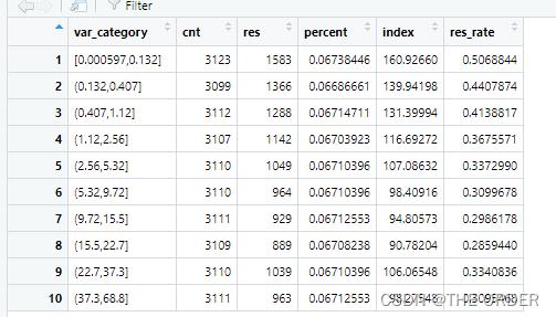
Encore une fois, les paires sont divisées en 10 Chaque ensemble de données est divisé en parts égales. liftCalcul, Comparer le rapport entre le nombre moyen d'applications à fort impact par groupe et le nombre total d'utilisateurs .Plus grand que100% Est l'étiquette du client au - dessus de la performance globale

nonmissing_perf<-within(prof2,
                        {res_rate<-res/cnt 
                        index<-res_rate/overall_resp_rate*100
                        percent<-cnt/overall_cnt
                        })  #add resp_rate,index,percent
View(nonmissing_perf)

#set missing_perf and non-missing_Perf together
View(missing_perf)
View(nonmissing_perf)
em_months_last_open_perf<-rbind(nonmissing_perf,missing_perf[,-1]) #set 2 data together
View(em_months_last_open_perf)

4 Valeurs manquantes,Traitement des valeurs aberrantes

1 Moins de3% Supprimer directement ou médiane ,Moyenne
2 3%——20%Supprimer ouknn,EM Retour à remplir
3 20%——50% Imputation multiple
4 50——80% Classification des valeurs manquantes
5 Supérieur à80%Jeter, Les données sont trop inexactes , L'analyse est très erronée

Les valeurs aberrantes sont généralement résolues par la méthode du capuchon

numeric variables

train$m2_em_count_valid <- ifelse(is.na(train$em_count_valid) == T, 2,      #when em_count_valid is missing ,then assign 2
                                  ifelse(train$em_count_valid <= 1, 1,         #when em_count_valid<=1 then assign 1
                                         ifelse(train$em_count_valid >=10, 10, #when em_count_valid>=10 then assign 10
                                                train$em_count_valid)))        #when 1<em_count_valid<10 and not missing then assign the raw value

summary(train$m2_em_count_valid)  #do a summary
summary(train$m1_EM_COUNT_VALID)  #do a summary

5 Ajustement du modèle

Sélectionner la variable la plus précieuse en fonction de l'entreprise

library(picante)  #call picante
var_list<-c('dv_response','m1_POS_NUM_ORDERS_24MO',
            'm1_POS_NUM_ORDERS',
            'm1_SH_MNTHS_LAST_INQUIRED',
            'm1_POS_SP_QTY_24MO',
            'm1_POS_REVENUE_TOTAL',
            'm1_POS_LAST_ORDER_DPA',
            'm1_POS_MARGIN_TOTAL',
            'm1_pos_mo_btwn_fst_lst_order',
            'm1_POS_REVENUE_BASE',
            'm1_POS_TOT_REVPERSYS',
            'm1_EM_COUNT_VALID',
            'm1_EM_NUM_OPEN_30',
            'm1_POS_MARGIN_TOTAL_12MO',
            'm1_EX_AUTO_USED0005_X5',
            'm1_SH_INQUIRED_LAST3MO',
            'm1_EX_AUTO_USED0005_X789',
            'm1_HH_INCOME',
            'm1_SH_INQUIRED_LAST12MO',
            'm1_POS_LAST_TOTAL_REVENUE',
            'm1_EM_ALL_OPT_OUT_FLAG',
            'm1_POS_REVENUE_TOTAL_6MO',
            'm1_EM_MONTHS_LAST_OPEN',
            'm1_POS_MNTHS_LAST_ORDER',
            'm1_WEB_MNTHS_SINCE_LAST_SES')  #put the variables you want to do correlation analysis here

Créer une matrice de coefficient de corrélation , Filtrer les variables dépendantes en fonction des dépendances , Méthode de la variable d'identification de sélection collinéaire ou méthode de la variable fictive ,logistic La régression peut être utilisée IV Variable de sélection de valeur

corr_var<-train[, var_list]  #select all the variables you want to do correlation analysis
str(corr_var)                #check the variable type
correlation<-data.frame(cor.table(corr_var,cor.method = 'pearson'))  #do the correlation
View(correlation)
cor_only=data.frame(row.names(correlation),correlation[, 1:ncol(corr_var)])  #select correlation result only
View(cor_only)

Fin de la sélection, Variables prêtes à être placées dans le modèle

var_list<-c('m1_WEB_MNTHS_SINCE_LAST_SES',
            'm1_POS_MNTHS_LAST_ORDER',
            'm1_POS_NUM_ORDERS_24MO',
            'm1_pos_mo_btwn_fst_lst_order',
            'm1_EM_COUNT_VALID',
            'm1_POS_TOT_REVPERSYS',
            'm1_EM_MONTHS_LAST_OPEN',
            'm1_POS_LAST_ORDER_DPA'
)   #put the variables you want to try in model here

mods<-train[,c(‘dv_response’,var_list)] #select Y and varibales you want to try
str(mods)
Ajustement non normalisé , La méthode de régression par étapes est utilisée pour sélectionner les variables après ajustement.

mods<-train[,c('dv_response',var_list)]  #select Y and varibales you want to try
str(mods)

(model_glm<-glm(dv_response~.,data=mods,family =binomial(link ="logit")))  #logistic model
model_glm
#Stepwise
library(MASS)
model_sel<-stepAIC(model_glm,direction ="both")  #using both backward and forward stepwise selection
model_sel
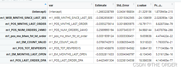
summary<-summary(model_sel)  #summary
model_summary<-data.frame(var=rownames(summary$coefficients),summary$coefficients) #do the model summary
View(model_summary)

Modélisation normalisée des données , La modélisation normalisée facilite la visualisation de chaque paire de variables yL'ampleur de l'impact

#variable importance
#standardize variable

#?scale
mods2<-scale(train[,var_list],center=T,scale=T) 
mods3<-data.frame(dv_response=c(train$dv_response),mods2[,var_list])
# View(mods3)
(model_glm2<-glm(dv_response~.,data=mods3,family =binomial(link ="logit")))  #logistic model
(summary2<-summary(model_glm2)) 
model_summary2<-data.frame(var=rownames(summary2$coefficients),summary2$coefficients) #do the model summary
View(model_summary2)
model_summary2_f<-model_summary2[model_summary2$var!='(Intercept)',]
model_summary2_f$contribution<-abs(model_summary2_f$Estimate)/(sum(abs(model_summary2_f$Estimate)))
View(model_summary2_f)

6 Évaluation du modèle

Régression ajustée VIFValeur

#Variable VIF
fit <- lm(dv_response~., data=mods)  #regression model
#install.packages('car')  #Install Package 'Car' to calculate VIF
require(car)  #call Car
vif=data.frame(vif(fit)) #get Vif
var_vif=data.frame(var=rownames(vif),vif) #get variables and corresponding Vif
View(var_vif)

Fabrication de matrices de coefficients de corrélation

#variable correlation
cor<-data.frame(cor.table(mods,cor.method = 'pearson')) #calculate the correlation
correlation<-data.frame(variables=rownames(cor),cor[, 1:ncol(mods)]) #get correlation only
View(correlation)

La production finale ROCCourbe, Dessiner un modèle ROCCourbe, Observez ses effets

library(ROCR)

#### test data####
pred_prob<-predict(model_glm,test,type='response') #predict Y
pred_prob
pred<-prediction(pred_prob,test$dv_response) #put predicted Y and actual Y together
pred@predictions
View(pred)
perf<-performance(pred,'tpr','fpr')   #Check the performance,True positive rate
perf
par(mar=c(5,5,2,2),xaxs = "i",yaxs = "i",cex.axis=1.3,cex.lab=1.4)  #set the graph parameter

#AUC value
auc <- performance(pred,"auc")
unlist(slot(auc,"y.values"))

#plotting the ROC curve
plot(perf,col="black",lty=3, lwd=3,main='ROC Curve')

#plot Lift chart
perf<-performance(pred,‘lift’,‘rpp’)
plot(perf,col=“black”,lty=3, lwd=3,main=‘Lift Chart’)

7 Répartition générale des groupes d'utilisateurs liftFig.

pred<-predict(model_glm,train,type='response')   #Predict Y
decile<-cut(pred,unique(quantile(pred,(0:10)/10)),labels=10:1, include.lowest = T)  #Separate into 10 groups
sum<-data.frame(actual=train$dv_response,pred=pred,decile=decile) #put actual Y,predicted Y,Decile together

decile_sum<-ddply(sum,.(decile),summarise,cnt=length(actual),res=sum(actual)) #group by decile
decile_sum2<-within(decile_sum,
                     {res_rate<-res/cnt 
                    index<-100*res_rate/(sum(res)/sum(cnt))
                     })  #add resp_rate,index
decile_sum3<-decile_sum2[order(decile_sum2[,1],decreasing=T),] #order decile
View(decile_sum3)

La Division décimale est utilisée , Segmentation des groupes de clients avec un nombre égal d'enregistrements ,On peut le découvrir.1-10 Utilisateurs hiérarchiques , Taux de réponse réel lift Ça vaut bien .
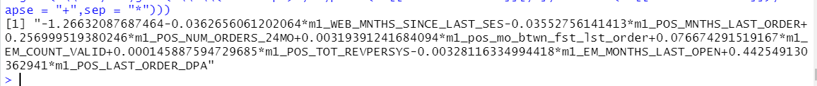
Coller l'équation de régression

ss <- summary(model_glm)  #put model summary together
ss
which(names(ss)=="coefficients")

#XBeta
#Y = 1/(1+exp(-XBeta))
#output model equoation
gsub("\\+-","-",gsub('\\*\\(Intercept)','',paste(ss[["coefficients"]][,1],rownames(ss[["coefficients"]]),collapse = "+",sep = "*")))