logistic回歸篇章

數據集接應上一節數據集合，本次的分析是從用戶是否為高響應用戶進行劃分，使用logistic回歸對用戶進行響應度預測，得到響應的概率。線性回歸，參考上一篇章

1 讀取和預覽數據

對數據進行加載讀取，數據依舊是脫敏數據，

file_path<-"data_response_model.csv" #change the location

# read in data
options(stringsAsFactors = F)
raw<-read.csv(file_path)   #read in your csv data
str(raw)     #check the varibale type
View(raw)    #take a quick look at the data
summary(raw) #take a quick look at the summary of variable

# response variable
View(table(raw$dv_response))  #Y
View(prop.table(table(raw$dv_response))) #Y frequency

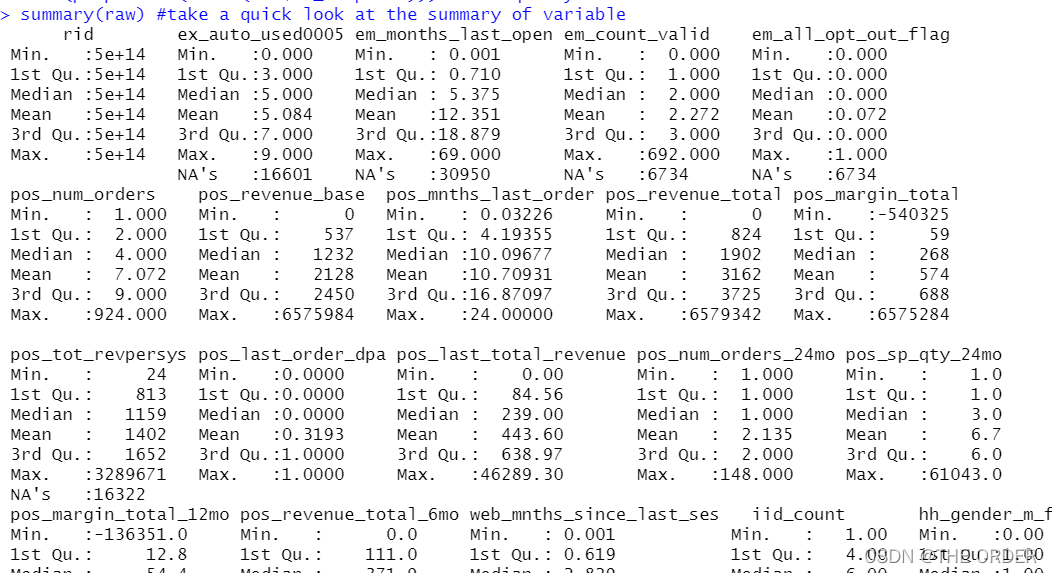
根據業務確定，數據的y值是響應率是dv_response，並觀察其情况

2 劃分數據

依舊把數據劃分為三部分，分別為訓練集，驗證集和測試集。

#Separate Build Sample
train<-raw[raw$segment=='build',]  #select build sample, it should be random selected when you build the model
View(table(train$segment))         #check segment
View(table(train$dv_response))     #check Y distribution  
View(prop.table(table(train$dv_response))) #check Y distribution

#Separate invalidation Sample
test<-raw[raw$segment=='inval',] #select invalidation(OOS) sample
View(table(test$segment))       #check segment
View(prop.table(table(test$dv_response))) #check Y distribution

#Separate out of validation Sample
validation<-raw[raw$segment=='outval',] #select out of validation(OOT) sample
View(table(validation$segment)) #check segment
View(prop.table(table(validation$dv_response))) #check Y distribution

3 profilng制作

對數據即中的響應率進行求和，原數據中高響應客戶為1，低響應客戶為0.求和的總數就是高響應客戶數，length就是總記錄數，求出其平均數即為總體平均數

# overall performance
overall_cnt=nrow(train)   #calculate the total count
overall_resp=sum(train$dv_response)  #calculate the total responders count
overall_resp_rate=overall_resp/overall_cnt  #calculate the response rate
overall_perf<-c(overall_count=overall_cnt,overall_responders=overall_resp,overall_response_rate=overall_resp_rate) #combine
overall_perf<-c(overall_cnt=nrow(train),overall_resp=sum(train$dv_response),overall_resp_rate=sum(train$dv_response)/nrow(train)) #combine
View(t(overall_perf))  #take a look at the summary

這裏做的劃分如同上一章節的劃分lift圖制作，也可用sql語句來寫，如同group by，計算出每組的平均響應率與總體響應率的比較。
在library之前，請先下載plyr包，寫sql需下載sqldf
install.packages(“sqldf”)

library(plyr)              #call plyr
?ddply
prof<-ddply(train,.(hh_gender_m_flag),summarise,cnt=length(rid),res=sum(dv_response)) #group by hh_gender_m_flg
View(prof)  #check the result
tt=aggregate(train[,c("hh_gender_m_flag","rid")],by=list(train[,c("hh_gender_m_flag")]),length) #group by hh_gender_m_flg
View(tt) 
#calculate the probablity
#prop.table(as.matrix(prof[,-1]),2)
#t(t(prof)/colSums(prof))

prof1<-within(prof,{res_rate<-res/cnt 
index<-res_rate/overall_resp_rate*100
percent<-cnt/overall_cnt
})  #add response_rate,index, percentage

View(prof1)   #check the result

library(sqldf)
#整型乘浮點型變浮點數據
sqldf("select hh_gender_m_flag,count() as cnt,sum(dv_response)as res,1.0sum(dv_response) /count(*) as res_rate from train group by 1 ")
缺失值也能作為特征的一部分，同樣可以對缺失值進行lift比較

nomissing<-data.frame(var_data[!is.na(var_data$em_months_last_open),])  #select the no missing value records 
missing<-data.frame(var_data[is.na(var_data$em_months_last_open),])     #select the missing value records

###################################### numeric Profiling:missing part   #############################################################

missing2<-ddply(missing,.(em_months_last_open),summarise,cnt=length(dv_response),res=sum(dv_response)) #group by em_months_last_open
View(missing2)  

missing_perf<-within(missing2,{res_rate<-res/cnt 
index<-res_rate/overall_resp_rate*100
percent<-cnt/overall_cnt
var_category<-c('unknown')
})   #summary

View(missing_perf)

這裏對非缺失值數據進行了劃分，將非缺失值數據，按照十分比特數劃分成了10等分。分別計算其總記錄數和總高響應客戶數量

nomissing_value<-nomissing$em_months_last_open  #put the nomissing values into a variable

#method1:equal frequency
nomissing$var_category<-cut(nomissing_value,unique(quantile(nomissing_value,(0:10)/10)),include.lowest = T)#separte into 10 groups based on records
class(nomissing$var_category)
View(table(nomissing$var_category))  #take a look at the 10 category

prof2<-ddply(nomissing,.(var_category),summarise,cnt=length(dv_response),res=sum(dv_response)) #group by the 10 groups
View(prof2)

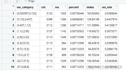
再次對劃分為10等分的數據每一組都進行lift計算，比較每組的平均高響應用戶數與總體的用戶數的比值。大於100%就是高於總體錶現的客戶標簽

nonmissing_perf<-within(prof2,
                        {res_rate<-res/cnt 
                        index<-res_rate/overall_resp_rate*100
                        percent<-cnt/overall_cnt
                        })  #add resp_rate,index,percent
View(nonmissing_perf)

#set missing_perf and non-missing_Perf together
View(missing_perf)
View(nonmissing_perf)
em_months_last_open_perf<-rbind(nonmissing_perf,missing_perf[,-1]) #set 2 data together
View(em_months_last_open_perf)

4 缺失值，异常值處理

1 少於3%直接删除或者中比特數，平均數填補
2 3%——20%删除或knn，EM回歸填補
3 20%——50% 多重插補
4 50——80%缺失值分類法
5 高於80%丟弃，數據太不准確了，分析失誤性很大

异常值通常用蓋帽法解决

numeric variables

train$m2_em_count_valid <- ifelse(is.na(train$em_count_valid) == T, 2,      #when em_count_valid is missing ,then assign 2
                                  ifelse(train$em_count_valid <= 1, 1,         #when em_count_valid<=1 then assign 1
                                         ifelse(train$em_count_valid >=10, 10, #when em_count_valid>=10 then assign 10
                                                train$em_count_valid)))        #when 1<em_count_valid<10 and not missing then assign the raw value

summary(train$m2_em_count_valid)  #do a summary
summary(train$m1_EM_COUNT_VALID)  #do a summary

5 模型擬合

根據業務選取最有價值的變量

library(picante)  #call picante
var_list<-c('dv_response','m1_POS_NUM_ORDERS_24MO',
            'm1_POS_NUM_ORDERS',
            'm1_SH_MNTHS_LAST_INQUIRED',
            'm1_POS_SP_QTY_24MO',
            'm1_POS_REVENUE_TOTAL',
            'm1_POS_LAST_ORDER_DPA',
            'm1_POS_MARGIN_TOTAL',
            'm1_pos_mo_btwn_fst_lst_order',
            'm1_POS_REVENUE_BASE',
            'm1_POS_TOT_REVPERSYS',
            'm1_EM_COUNT_VALID',
            'm1_EM_NUM_OPEN_30',
            'm1_POS_MARGIN_TOTAL_12MO',
            'm1_EX_AUTO_USED0005_X5',
            'm1_SH_INQUIRED_LAST3MO',
            'm1_EX_AUTO_USED0005_X789',
            'm1_HH_INCOME',
            'm1_SH_INQUIRED_LAST12MO',
            'm1_POS_LAST_TOTAL_REVENUE',
            'm1_EM_ALL_OPT_OUT_FLAG',
            'm1_POS_REVENUE_TOTAL_6MO',
            'm1_EM_MONTHS_LAST_OPEN',
            'm1_POS_MNTHS_LAST_ORDER',
            'm1_WEB_MNTHS_SINCE_LAST_SES')  #put the variables you want to do correlation analysis here

制作相關系數矩陣，根據相關性篩選變量相關的，共線性選擇標識變量法或啞變量法，logistic回歸可使用IV值選擇變量

corr_var<-train[, var_list]  #select all the variables you want to do correlation analysis
str(corr_var)                #check the variable type
correlation<-data.frame(cor.table(corr_var,cor.method = 'pearson'))  #do the correlation
View(correlation)
cor_only=data.frame(row.names(correlation),correlation[, 1:ncol(corr_var)])  #select correlation result only
View(cor_only)

選擇完，准備放到模型裏面的變量

var_list<-c('m1_WEB_MNTHS_SINCE_LAST_SES',
            'm1_POS_MNTHS_LAST_ORDER',
            'm1_POS_NUM_ORDERS_24MO',
            'm1_pos_mo_btwn_fst_lst_order',
            'm1_EM_COUNT_VALID',
            'm1_POS_TOT_REVPERSYS',
            'm1_EM_MONTHS_LAST_OPEN',
            'm1_POS_LAST_ORDER_DPA'
)   #put the variables you want to try in model here

mods<-train[,c(‘dv_response’,var_list)] #select Y and varibales you want to try
str(mods)
非標准化擬合，擬合後再使用逐步回歸法進行篩選變量

mods<-train[,c('dv_response',var_list)]  #select Y and varibales you want to try
str(mods)

(model_glm<-glm(dv_response~.,data=mods,family =binomial(link ="logit")))  #logistic model
model_glm
#Stepwise
library(MASS)
model_sel<-stepAIC(model_glm,direction ="both")  #using both backward and forward stepwise selection
model_sel
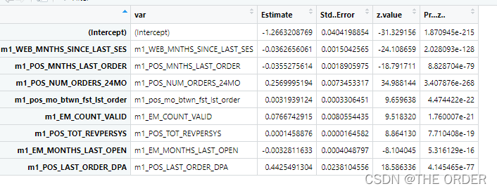
summary<-summary(model_sel)  #summary
model_summary<-data.frame(var=rownames(summary$coefficients),summary$coefficients) #do the model summary
View(model_summary)

對數據進行標准化後的建模，標准化的建模方便查看每個變量對y的影響程度

#variable importance
#standardize variable

#?scale
mods2<-scale(train[,var_list],center=T,scale=T) 
mods3<-data.frame(dv_response=c(train$dv_response),mods2[,var_list])
# View(mods3)
(model_glm2<-glm(dv_response~.,data=mods3,family =binomial(link ="logit")))  #logistic model
(summary2<-summary(model_glm2)) 
model_summary2<-data.frame(var=rownames(summary2$coefficients),summary2$coefficients) #do the model summary
View(model_summary2)
model_summary2_f<-model_summary2[model_summary2$var!='(Intercept)',]
model_summary2_f$contribution<-abs(model_summary2_f$Estimate)/(sum(abs(model_summary2_f$Estimate)))
View(model_summary2_f)

6 模型評估

回歸擬合的VIF值

#Variable VIF
fit <- lm(dv_response~., data=mods)  #regression model
#install.packages('car')  #Install Package 'Car' to calculate VIF
require(car)  #call Car
vif=data.frame(vif(fit)) #get Vif
var_vif=data.frame(var=rownames(vif),vif) #get variables and corresponding Vif
View(var_vif)

相關系數矩陣制作

#variable correlation
cor<-data.frame(cor.table(mods,cor.method = 'pearson')) #calculate the correlation
correlation<-data.frame(variables=rownames(cor),cor[, 1:ncol(mods)]) #get correlation only
View(correlation)

最後制作ROC曲線，對模型畫ROC曲線圖，觀察其效果

library(ROCR)

#### test data####
pred_prob<-predict(model_glm,test,type='response') #predict Y
pred_prob
pred<-prediction(pred_prob,test$dv_response) #put predicted Y and actual Y together
pred@predictions
View(pred)
perf<-performance(pred,'tpr','fpr')   #Check the performance,True positive rate
perf
par(mar=c(5,5,2,2),xaxs = "i",yaxs = "i",cex.axis=1.3,cex.lab=1.4)  #set the graph parameter

#AUC value
auc <- performance(pred,"auc")
unlist(slot(auc,"y.values"))

#plotting the ROC curve
plot(perf,col="black",lty=3, lwd=3,main='ROC Curve')

#plot Lift chart
perf<-performance(pred,‘lift’,‘rpp’)
plot(perf,col=“black”,lty=3, lwd=3,main=‘Lift Chart’)

7 總體劃分用戶群lift圖

pred<-predict(model_glm,train,type='response')   #Predict Y
decile<-cut(pred,unique(quantile(pred,(0:10)/10)),labels=10:1, include.lowest = T)  #Separate into 10 groups
sum<-data.frame(actual=train$dv_response,pred=pred,decile=decile) #put actual Y,predicted Y,Decile together

decile_sum<-ddply(sum,.(decile),summarise,cnt=length(actual),res=sum(actual)) #group by decile
decile_sum2<-within(decile_sum,
                     {res_rate<-res/cnt 
                    index<-100*res_rate/(sum(res)/sum(cnt))
                     })  #add resp_rate,index
decile_sum3<-decile_sum2[order(decile_sum2[,1],decreasing=T),] #order decile
View(decile_sum3)

采用的是十分比特數劃分，等記錄數的劃分客戶群體，可以發現1-10個層次的用戶，真實響應率lift值不錯。
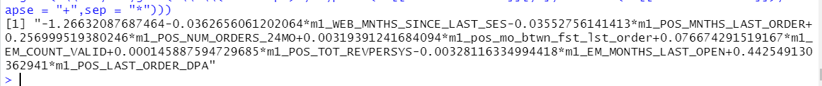
將回歸方程貼出來

ss <- summary(model_glm)  #put model summary together
ss
which(names(ss)=="coefficients")

#XBeta
#Y = 1/(1+exp(-XBeta))
#output model equoation
gsub("\\+-","-",gsub('\\*\\(Intercept)','',paste(ss[["coefficients"]][,1],rownames(ss[["coefficients"]]),collapse = "+",sep = "*")))