Deep learning notes ( Two )—— Principle and implementation of activation function

gossip

Yesterday, I pushed down the cross entropy in detail , I think it's OK , Continue to refuel today .

ReLU

principle

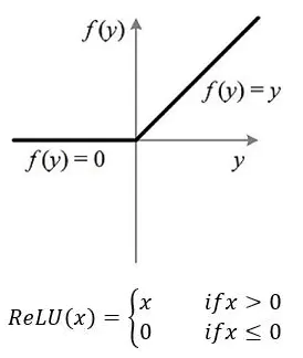
Definition ：ReLU Is a modified linear element (rectified linear unit), stay 0 and x Take the maximum value between .
Reasons for appearance ： because sigmoid and tanh Gradients tend to disappear , To train deep neural networks , Need an activation function neural network , It looks and behaves like a linear function , But it's actually a nonlinear function , Allows you to learn complex relationships in data . The function must also provide more sensitive activation and input , Avoid saturation . and ReLU yes Unsaturated activation function , Gradient disappearance is not easy to occur .

def ReLU(input):
	if input>0:
		return input
	else:
		return 0

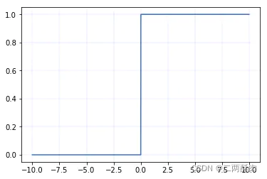
ReLU Function expression for ：
When x <= 0 when ,ReLU = 0
When x > 0 when ,ReLU = x

ReLU Derivative expression of ：
When x<= 0 when , Derivative is 0
When x > 0 when , Derivative is 1

advantage

Simple calculation

because ReLU Just one max() Function can complete the operation , and tanh and sigmoid Exponential operation is required , therefore ReLU The calculation cost is very low .

The representation is sparse

ReLU True zero value can be output when negative input , Allow the hidden layer in the neural network to contain one or more true zero values , This is called sparse representation . It means learning , Because it can speed up learning and simplify models . Effectively alleviate the problem of over fitting , because ReLU It is possible to change the output of some nerve nodes into 0, This leads to the death of nerve nodes , It reduces the complexity of neural network .

Linear behavior

When the input is greater than zero ,ReLU It looks like a linear function , When the network behavior is nearly linear , Easier to optimize , There will be no gradient disappearance or gradient explosion , When x Greater than 0 when ,ReLU The gradient of is constant 1, The gradient will not become smaller or larger as the network depth deepens , Thus, no gradient disappearance or gradient explosion will occur , Therefore, it can be more suitable for training deep network . Now in deep learning , The default activation function is ReLU.

shortcoming

Not suitable for RNN Class network

Yes MLPs,CNNs Use ReLU, But it's not RNNs.ReLU It can be used in most types of neural networks , It is usually used as the activation function of multilayer perceptron neural network and convolutional neural network . Traditionally ,LSTMs Use tanh Activate function to activate cell state , Use Sigmoid Activate function as node Output . and ReLU Usually not suitable for RNN Use of type network .

Code

import torch
import torch.nn as nn

relu = nn.ReLU(inplace=True)

---

Sigmoid

principle

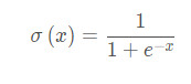
Sigmoid It's a common nonlinear activation function , You can map all real numbers to （0, 1） On interval , It uses nonlinear method to normalize the data ;sigmoid Functions are usually used in Regression prediction and binary classification （ That is, according to whether it is greater than 0.5 To classify ） In the output layer of the model .

Function formula ：

def Sigmoid(x):
    return 1. / (1 + np.exp(-x))

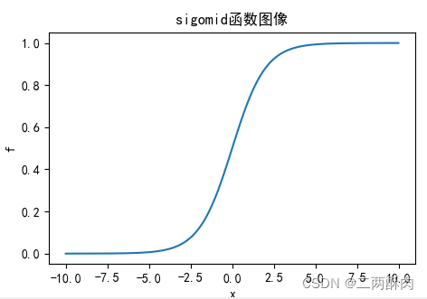
diagram ：

derivative ：

Derivative image ：

advantage

Derivative easily

Gradient smoothing , Derivative easily

Optimization and stability

Sigmoid The output of the function is mapped to (0,1) Between , Monotone continuous , Limited output range , Optimization and stability , Can be used as output layer

shortcoming

Large amount of computation

Both forward propagation and back propagation contain power operation and division , Therefore, there are large computing resources .

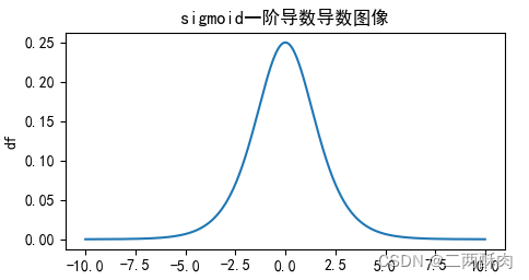
The gradient disappears

The gradient disappears ： Enter a larger or smaller value （ Both sides of the image ） when ,sigmoid The derivative is close to zero , So in back propagation , This local gradient will be multiplied by the gradient of the whole cost function with respect to the output of the unit , The result will also be close to 0 , The purpose of updating parameters cannot be achieved ;

This can be seen from its derivative image , If we initialize the neural network with a weight of [0,1] [0,1][0,1] The random value between , It can be seen from the mathematical derivation of back propagation algorithm , When the gradient propagates from back to front , The gradient value of each transfer layer will be reduced to the original 0.25 times , If there are many hidden layers in neural network , Then the gradient will become very small and close to 0, That is, the gradient disappears ;

Code

import torch
import torch.nn as nn
sigmoid=nn.Sigmoid()

---

Softmax

principle

Sigmoid Function can only handle two categories , This does not apply to multi classification problems , therefore Softmax Can solve this problem effectively .Softmax Functions are often used in the last layer of neural networks , Make the probability value of each category in (0, 1) Between .Softmax = Multi category classification problem = There is only one correct answer = Mutually exclusive output （ For example, handwritten numbers , Iris ）. Building classifiers , When solving a problem with only one correct answer , use Softmax The function processes the raw output values .Softmax The denominator of the function synthesizes all the factors of the original output value , It means ,Softmax The different probabilities obtained by the function are related to each other . That is, the sum of all the probabilities obtained is 1, The example looks at the code section

def softmax(x):
    return np.exp(x) / sum(np.exp(x))

advantage

It has a wide range of applications

Compare with sigmoid,softmax Can deal with multiple categories , Therefore, it can be applied to more fields .

Open the gap between values

because Softmax The function first widens the difference between the elements of the input vector （ By exponential function ）, And then normalized to a probability distribution , When applied to classification problems , It makes the probability difference of each category more significant , The probability of maximum production is closer to 1, In this way, the output distribution is closer to the real distribution . Because it opens the gap , This is convenient to improve loss, Can get more learning results .

Code

give an example ：
Suppose a three class dataset of chickens, ducks and geese , If one batch There are three inputs , Through the previous network , The result is （[10,8,6],[7,9,5],[5,4,10]).
The actual tag value is [0,1,2], That is, chicken, duck and goose .
Means ： The network speculates that the probability of chicken is [86.68%], duck [11.73%], goose [1.59%], The last two lines are the same .

import torch 
import torch.nn as nn
import math
import time
#  Suppose it turns out that 
input_1=torch.Tensor([0,1,2])
#  Predicted results 
input_2 = torch.Tensor([
                        [10,8,6],
                        [7,9,5],
                        [5,4,10]
                        ])
# Specify... In different directions softmax
softmax = nn.Softmax(dim=1)
# Tensor experiments on different dimensions 
output = softmax(input_2)
print(output)
#------------#
#tensor([[0.8668, 0.1173, 0.0159],
# [0.1173, 0.8668, 0.0159],
# [0.0067, 0.0025, 0.9909]])
#------------#

---

Tanh

principle

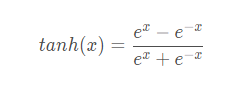
The formula ：

def tanh(x):
    return np.sinh(x)/np.cosh(x)

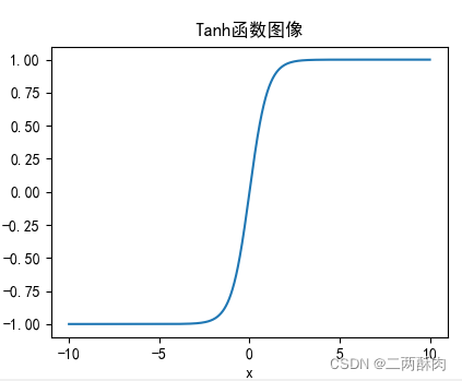
Function image

Function form after first-order derivation ：

Derivative function image ：

advantage

Fast convergence

Than Sigmoid Function converges faster

The gradient vanishing problem is lighter

tanh(x) Gradient vanishing problem ratio sigmoid Be light . Because you can see ,sigmoid In the near 0 Each layer will shrink 0.25 times , and tanh Be accessible to 1, So in deep networks , The gradient vanishing problem is alleviated .

Output to 0 Centered

comparison Sigmoid function , The output is in the form of 0 Centered zero-centered

shortcoming

The calculation consumption is large

It can be seen that it has carried out several exponential operations , It consumes a relatively large calculation cost .

The gradient disappears and still exists

As can be seen from the derivative image , Its derivative image and sigmoid There are great similarities , Still unchanged Sigmoid The biggest problem with functions —— The gradient due to saturation disappears .

Code

import torch
import torch.nn as nn

relu = nn.tanh()

---

LeakyReLU

principle

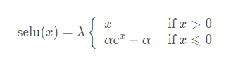
Leaky ReLU To solve “ ReLU Death ” An attempt at a problem . Mainly to avoid death ReLU:x Less than 0 When , The derivative is a small number , instead of 0.

Usually a by 0.01.

def ReLU(input):
	if input>0:
		return input
	else:
		return 0.01*input

advantage

Low computing cost

Fast calculation ： Does not include exponential operations .

Can get a negative output

Compare with ReLU You can get a negative output

Have ReLU Other benefits

shortcoming

a It's a super parameter. , It needs to be set manually

Both parts are linear

Code

import torch
import torch.nn as nn

LR=nn.LeakyReLU(inplace=True)

---

ReLU6

principle

Mainly for the mobile terminal float16 When the precision is low , It also has good numerical resolution , If the ReLu The output value of is unlimited , Then the output range is 0 To infinity , And low precision float16 Its value cannot be accurately described , Bring precision loss .

characteristic

Basic and ReLU identical , Only the upper limit of the output value is limited .

def ReLU(input):
	if input>0:
		return min(6,input)
	else:
		return 0

Code

"""pytorch  neural network """
import torch.nn as nn
Re=nn.ReLU6(inplace=True)

---

ELU

principle

LU It also solves the problem of ReLU The problem of . And ReLU comparison ,ELU There is a negative value , This brings the average value of activation close to zero . Mean activation close to zero can make learning faster , Because they make gradients closer to natural gradients .

Function image ：

advantage

It's solved Dead ReLU

No, Dead ReLU problem , Close to the average output 0, With 0 Centered .

Speed up learning

ELU By reducing the effect of offset , Make the normal gradient closer to the unit natural gradient , So that the mean value can be accelerated to zero .

Reduce variation and information

ELU The function saturates to a negative value with a small input , So as to reduce the forward propagation of variation and information .

shortcoming

The amount of calculation becomes larger

ELU Functions are more computationally intensive . And Leaky ReLU similar , Although theoretically better than ReLU It is better to , But at present, there is no sufficient evidence in practice to show that ELU It's always better than ReLU good .

Code

import torch
import torch.nn as nn

LR=nn.ELU()

# ELU Function in numpy The realization of 

import numpy as np
import matplotlib.pyplot as plt

def elu(x, a):
    y = x.copy()
    for i in range(y.shape[0]):
        if y[i] < 0:
            y[i] = a * (np.exp(y[i]) - 1)
    return y
if __name__ == '__main__':
    x = np.linspace(-50, 50)
    a = 0.5
    y = elu(x, a)
    print(y)
    plt.plot(x, y)
    plt.title('elu')
    plt.axhline(ls='--',color = 'r')
    plt.axvline(ls='--',color = 'r')
    # plt.xticks([-60,60]),plt.yticks([-10,50])
    plt.show()

---

SELU

principle

SELU From the paper Self-Normalizing Neural Networks, The author is Sepp Hochreiter,ELU Also from their group .
SELU In fact, that is ELU ride lambda, The point is this lambda It is greater than 1 Of , It's given in the paper lambda and alpha Value ：

• lambda = 1.0507
• alpha = 1.67326

Function image ：

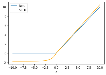
advantage

Self normalization

SELU Activation can self normalize the neural network （self-normalizing）;

No gradient disappearance or explosion

There is no possibility of gradient disappearance or explosion , The theorem in the appendix of the paper 2 and 3 Provided proof that .

shortcoming

Less application

Less application , Need more validation ;

It needs to be initialized

lecun_normal and Alpha Dropout： need lecun_normal Initialize the weight ; If dropout, You have to use Alpha Dropout Special version of .

Code

import torch
import torch.nn as nn

SELU=nn.SELU()

---

Parametric ReLU (PRELU)

principle

Formally and Leak_ReLU Similar in form , The difference is ：PReLU Parameters of alpha It's learnable , Need to update according to gradient .

• alpha=0： Degenerate to ReLU
• alpha Fixed not updated , Degenerate to Leak_ReLU
  

advantage

And ReLU identical .

shortcoming

In different problems , Different performances .

Code

import torch
import torch.nn as nn

PReLU= nn.PReLU()

---

Gaussian Error Linear Unit(GELU)

principle

Gaussian error linear element activation function in the recent Transformer Model （ Google's BERT and OpenAI Of GPT-2） It has been applied to .GELU My paper comes from 2016 year , But it has only recently attracted attention .

advantage

The effect is good

It seems to be NLP The current best in the field ; Especially in Transformer The best model ;

Avoid gradients disappearing

It can avoid the problem of gradient disappearance .

shortcoming

This 2016 The novel activation function proposed in still lacks the test of practical application .

Code

import torch
import torch.nn as nn
gelu_f== nn.GELU()

import torch
import torch.nn as nn
import torch.nn.functional as F
import numpy as np
from matplotlib import pyplot as plt

class GELU(nn.Module):
    def __init__(self):
        super(GELU, self).__init__()

    def forward(self, x):
        return 0.5*x*(1+F.tanh(np.sqrt(2/np.pi)*(x+0.044715*torch.pow(x,3))))

def gelu(x):
    return 0.5*x*(1+np.tanh(np.sqrt(2/np.pi)*(x+0.044715*np.power(x,3))))

x = np.linspace(-4,4,10000)
y = gelu(x)
plt.plot(x, y)
plt.show()

---

Swish

principle

Swish The activation function was born in Google Brain 2017 The paper of Searching for Activation functions in , The definition for ：

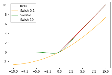
β Is a constant or trainable parameter .
Swish The effect on the deep model is better than ReLU. for example , Only use Swish Unit replacement ReLU Can handle Mobile NASNetA stay ImageNet Upper top-1 The classification accuracy is improved 0.9%,Inception-ResNet-v The classification accuracy of 0.6%.

characteristic

Swish There is no upper bound, there is a lower bound 、 smooth 、 Nonmonotonic properties .

Code

import torch
import torch.nn as nn
class Swish(nn.Module):
    def __init__(self):
        super(Swish, self).__init__()
 
    def forward(self, x):
        x = x * F.sigmoid(x)
        return x

Swi=Swish()

---

Function derivation drawing code

 Yes 
import sympy as sy	# It is used for mathematical calculations such as derivative and integral 
import matplotlib.pyplot as plt	# mapping 
import numpy as np

x = sy.symbols('x')	# Define symbolic variables x
#sigmoid function 
f = 1. / (1 + sy.exp(-x)) 
df = sy.diff(f,x)	# Find the first derivative 
#ddf = sy.diff(df,x)
ddf = sy.diff(f,x,2)	# Take the second derivative , Parameters 2 Is the order of derivation 

# Create an empty list to save data 
x_value = []	# Save arguments x The value of 
f_value = []	# Save function values f The value of 
df_value = []	# Save the first derivative df The value of 

for i in np.arange(-10,10,0.01):
    x_value.append(i)# Yes x Carry out the value 
    f_value.append(f.subs('x',i))# take i Value into the expression 
    df_value.append(df.subs('x',i))# take i Value into the derivation expression 


# It takes two lines of code to display Chinese normally 
plt.rcParams['font.sans-serif']=['SimHei']
plt.rcParams['axes.unicode_minus']=False


plt.title('sigomid Function image ')
plt.xlabel('x')
plt.ylabel('f')
plt.plot(x_value,f_value)
plt.show()

plt.title('sigmoid First derivative image ')
plt.xlabel('x')
plt.ylabel('df')
plt.plot(x_value,df_value)
plt.show()