Detailed explanation of split canvas function

One . Preface

In the use of matplotlib In the process of data visualization , We are inseparable from an important carrier – canvas （Figure）. One Figure Object is the top-level container for all drawing elements , Want to realize the rational use of canvas , Partition use is essential .

---

First of all, understand the concept of sub area , As the name suggests, the sub area is to put the big canvas （FIgure） Divided into several sub canvases , These sub canvases form the drawing area , Its essence is to add coordinate axis system to the crisscross row and column grid . Next, I will mainly introduce 3 A correlation function , All the example codes in the following are in Ipython Implemented on , And the related library import and Chinese modification statements have been omitted , The method mentioned in this paper is equivalent to function .

---

Two .subplots function

This function is the simplest and most direct , call plt.subplots() Will directly create a 1 That's ok 1 Grid layout subinterval of column , Create a Figure object .

2.1 Function definition

subplots(nrows=1, 
		ncols=1, 
		*, 
		sharex=False,
		sharey=False, 
		squeeze=True, 
		subplot_kw=None, 
		gridspec_kw=None, 
		fig_kw)

Parameter description ：

Parameters 1：nrows： Integer type , Specify the number of rows in the subgraph grid

Parameters 2：ncols： Integer type , Specify the number of columns in the subgraph grid

Parameters 3：sharex： Boolean or character , Specify whether to share x Axis , Optional {‘none’,‘all’,‘row’,‘col’}

​ none： Equate to False, Specifies that all subgraphs are not shared

​ all： Appoint x Axis or y The axis will be shared among all subgraphs

​ row： Specifies that each row of subgraphs will share a x Axis or y Axis

​ col： Specifies that each column of subgraphs will share a x Axis or y Axis

Parameters 4：sharey： Boolean or character , Specify whether to share y Axis , Optional {‘none’,‘all’,‘row’,‘col’}

​ none： Equate to False, Specifies that all subgraphs are not shared

​ all： Appoint x Axis or y The axis will be shared among all subgraphs

​ row： Specifies that each row of subgraphs will share a x Axis or y Axis

​ col： Specifies that each column of subgraphs will share a x Axis or y Axis

Parameters 5：squeeze： Boolean type , Specify whether to compress

Parameters 6：subplot_kw： Dictionary type , Pass to add_subplot Method , Specify the key parameters of the call to create each subgraph

Parameters 7：gridspec_kw： Dictionary type , Pass to GridSpec class , Specify the keyword parameters of the grid placed by the subgraph

Parameters 8：**fig_kw： Dictionary type , Pass to pyplot.figure Method

Return value 1：FIgure example

Return value 2：Axes Example or Axes Instance array , The array has the same shape as the grid

---

Parameters, ：

1. fig_kw Parameters passed to pyplot.figure Method means that all the contents of the parameter will be passed directly to plt.figure Method .subplot_kw、subplot_kw Empathy .
2. For parameters squeeze, If True And construct only one subgraph , Returns a single Axes Object will be returned as a scalar . about Nx1 or 1xM Subgraphs , The returned object contains Axes Object's numpy Array . about N×M individual , Sub district and N> 1 and M> 1 Return to 2D array . If False, No compression at all ： Back to Axes Objects always contain Axes Example of 2D Array , Even if it turns out to be 1x1. See below for specific examples .

---

2.2 Function explanation

The advantage of this function is that it can be done in one step , establish Figure Object while creating the grid layout of the specified rows and columns , A lot less code . The following is the internal implementation of this function ：

fig = figure(fig_kw)	# establish Figure object 
axs = fig.subplots(nrows=nrows, 	# Designated line 
					ncols=ncols, 	# Specified column 
					sharex=sharex, 	# Specify whether to share X Axis 
					sharey=sharey,	# Specify whether to share y Axis 
                    squeeze=squeeze, 	# Specifies whether to compress the return value 
                    subplot_kw=subplot_kw,	
                    gridspec_kw=gridspec_kw)
return fig, axs	# return Figure Object and coordinate system 

You can see the call plt.figure Function and pass arguments fig_kw And create a Figure object , This is what I said above to pass on to plt.figure Function means . Then call Figure.subplots Method to create grid layout and coordinate axis system . Here is fig.subplots Core code ：

  if self.get_constrained_layout():
  		gs = GridSpec(nrows, ncols, figure=self, gridspec_kw)	# establish GridSpec Class instance 
  else:
        # this should turn constrained_layout off if we don't want it
        gs = GridSpec(nrows, ncols, figure=None, gridspec_kw)
  self._gridspecs.append(gs)

  # Create array to hold all axes.
  axarr = np.empty((nrows, ncols), dtype=object)	# Create an empty matrix , Type is object 
  # Cycle to create a coordinate system , Subscript 0 Start 
  for row in range(nrows):
  		for col in range(ncols):
        	shared_with = {
    "none": None, "all": axarr[0, 0],"row": axarr[row, 0], "col": axarr[0, col]}	#sharex and sharey Check your dictionary 
            subplot_kw["sharex"] = shared_with[sharex]	# Dictionary values 
            subplot_kw["sharey"] = shared_with[sharey]	# Dictionary values 
            axarr[row, col] = self.add_subplot(gs[row, col], subplot_kw)	# Create a coordinate system 
# turn off redundant tick labeling
	# Setup and share X Axis 
  if sharex in ["col", "all"]:
    # turn off all but the bottom row
  	for ax in axarr[:-1, :].flat:
    	ax.xaxis.set_tick_params(which='both', labelbottom=False, labeltop=False)
        ax.xaxis.offsetText.set_visible(False)
  # Setup and share Y Axis 
  if sharey in ["row", "all"]:
  	# turn off all but the first column
    for ax in axarr[:, 1:].flat:
    	ax.yaxis.set_tick_params(which='both', labelleft=False, labelright=False)
        ax.yaxis.offsetText.set_visible(False)
        
  if squeeze:
  		return axarr.item() if axarr.size == 1 else axarr.squeeze()	# call squeeze Delete one-dimensional pressing method 
  else:
        return axarr	# Returns a two-dimensional matrix 

First create GridSpec Class instance , This class is used to specify the geometry of the mesh . Then cycle through the creation of the coordinate system , And add it to an empty matrix , here squeeze Parameters and have an effect , The return value is a two-dimensional matrix of the specified shape , The next two if-for The code block is used to set sharex and sharey Parameter response . Finally, squeeze Parameter detection , Assuming that True Return a pure instance or a two-dimensional matrix according to the number of rows and columns , Assuming that False Returns a two-dimensional matrix anyway .

---

2.3 Example of function

2.3.1squeeze Parameter example

First create a 1 That's ok 1 Grid layout of columns ,squeeze Parameter is False, Look at its return value ：

fig, ax = plt.subplots(squeeze=False)
ax.shape, ax

The result is as follows ：

((1, 1), array([[<AxesSubplot:>]], dtype=object))

The proof returns a binary array , Not an object , The following will squeeze The parameter is changed to True：

fig, ax = plt.subplots(squeeze=True)
ax

The result is as follows ：

<AxesSubplot:>

The return value is simply an object . But what if we set multiple rows or columns ？

fig, ax2 = plt.subplots(2, 2, squeeze=True)
ax2.shape, ax2

fig, ax1 = plt.subplots(2, 2, squeeze=False)
ax1.shape, ax1

The result is as follows ：

((2, 2),
 array([[<AxesSubplot:>, <AxesSubplot:>],
        [<AxesSubplot:>, <AxesSubplot:>]], dtype=object))
        
((2, 2),
 array([[<AxesSubplot:>, <AxesSubplot:>],
        [<AxesSubplot:>, <AxesSubplot:>]], dtype=object))        

Prove that in the case of multiple rows and columns ,squeeze It doesn't matter .

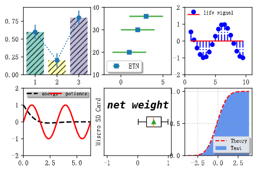
2.3.2 Comprehensive examples

fig, ax = plt.subplots(2, 3)

colors_list = ['#8dd3c7', '#ffffb3', '#bebada']
ax[0, 0].bar([1, 2, 3], [0.6, 0.2, 0.8], color=colors_list, width=0.8, hatch='///', align='center')
ax[0, 0].errorbar([1, 2, 3], [0.6, 0.2, 0.8], yerr=0.1, capsize=0, ecolor='#377eb8', fmt='o:')

ax[0, 1].errorbar([1, 2, 3], [20, 30, 36], xerr=2, ecolor='#4daf4a', elinewidth=2, fmt='s', label='ETN')
ax[0, 1].legend(loc=3, fancybox=True, shadow=True, fontsize=10, borderaxespad=0.4)
ax[0, 1].set_ylim(10, 40)
ax[0, 1].set_xlim(-2, 6)

x3 = np.arange(1, 10, 0.5)
y3 = np.cos(x3) 

ax[0, 2].stem(x3, y3, basefmt='r-', linefmt='b-.', markerfmt='bo', label='life signal')
ax[0, 2].legend(loc=2, fancybox=True, shadow=True, frameon=False, fontsize=8, borderaxespad=0.6, borderpad=0.0)
ax[0, 2].set_ylim(-2, 2)
ax[0, 2].set_xlim(0, 11)

x4 = np.linspace(0, 2*np.pi, 500)
x4_1 = np.linspace(0, 2*np.pi, 1000)
y4 = np.cos(x4)*np.exp(-x4)
y4_1 = np.sin(2*x4_1)
line1, line2 = ax[1, 0].plot(x4, y4, 'k--', x4_1, y4_1, 'r-', lw=2)
ax[1, 0].legend((line1, line2), ('energy', 'patience'), loc=2, fancybox=True, shadow=True, framealpha=0.3,mode='expand', fontsize=8, ncol=2, columnspacing=2, borderpad=0.1, markerscale=0.1)
ax[1, 0].set_ylim(-2, 2)
ax[1, 0].set_xlim(0, 2*np.pi)

x5 = np.random.rand(100)
ax[1, 1].boxplot(x5, vert=False, showmeans=True, meanprops=dict(color='black'))
ax[1, 1].set_yticks([])
ax[1, 1].set_xlim(-1.1, 1.1)
ax[1, 1].set_ylabel('Miscro SD Card')
ax[1, 1].text(-1.0, 1.2, 'net weight', fontsize=15, style='italic', weight='black', family='monospace')

mu = 0.0
sigma = 1.0

x6 = np.random.randn(10000)
n, bins, patches = ax[1, 2].hist(x6, bins=30, histtype='stepfilled', cumulative=True, color='cornflowerblue', 
label='Test', density=True)
y = ((1 / (np.sqrt(2 * np.pi) * sigma)) * np.exp(-0.5 * (1 / sigma * (bins-mu))  2))
y = y.cumsum()
y /= y[-1]

ax[1, 2].plot(bins, y, 'r--', lw=1.5, label='Theory')
ax[1, 2].set_ylim([0.0, 1.1])
ax[1, 2].grid(ls=':', lw=1, color='grey', alpha=0.5)
ax[1, 2].legend(fontsize=8, shadow=True, fancybox=True, framealpha=0.8)
ax[1, 2].autoscale()

plt.show()

The result is as follows ：

---

3、 ... and .plt.subplot function

This function is a pair of Figure.add_subplot Packaging of methods , Its purpose is to add the axis to the existing Figure object , Or retrieve an existing axis , Its core statement is fig = gcf() Get current Figure object .

3.1 Function definition

subplot There are many forms , Some examples are as follows ：

subplot(nrows, ncols, index, kwargs)
subplot(pos, kwargs)
subplot(kwargs)
subplot(ax)

Parameter description ：

Parameters 1：* args： Specify the method of describing the subgraph

​ （nrows,ncols,index）： Specify the number of lines 、 The number of columns and the index of the currently active subgraph , Index from the top left corner 1 Start and increase to the right . The index can also be specified as a two element tuple （start, end） , That is, draw a cross region subgraph

​ Three digit integer ： Hundred bit 、 ten 、 Each bit specifies the number of rows 、 Number of columns and index , Only if the number of subgraphs does not exceed 9 Use only after a period of time .

Parameters 2：projection： Specify the axis projection ,{None,“ aitoff”,“ hammer”,“ lambert”,“ mollweide”,“ polar”,“ rectalinear”,str}

Parameters 3：polar： Boolean type , Specify whether to use projection=‘polar’, That is, use the polar coordinate system

Parameters 4：sharex： Specify whether to share X Axis

Parameters 5：sharey： Specify whether to share Y Axis

Parameters 6：label： Specify the axis label

Return value ： Returns the axis base class based on the specified projection method

---

Parameters, ：

1. polar Try not to use this parameter , All projection parameters are best used projection Parameters to transmit .
2. When using this function, the index subscripts are from 1 Start . instead of 0, Bear in mind ！！！

---

3.2 Function explanation

Here are subplot Internal implementation of function ：

fig = gcf()	# call plt.gcf Get the current Figure object 

# First, search for an existing subplot with a matching spec.
key = SubplotSpec._from_subplot_args(fig, args)

# Retrieve the existing coordinate system 
for ax in fig.axes:
    # if we found an axes at the position sort out if we can re-use it
    if hasattr(ax, 'get_subplotspec') and ax.get_subplotspec() == key:
        # if the user passed no kwargs, re-use
        if kwargs == {
    }:
            break
        # if the axes class and kwargs are identical, reuse
        elif ax._projection_init == fig._process_projection_requirements(
        *args, **kwargs):
                break
		else:
    		# we have exhausted the known Axes and none match, make a new one!
    		ax = fig.add_subplot(*args, **kwargs)	# If there is no match, the corresponding subgraph will be created according to the parameters 

fig.sca(ax)	# Sets the current axis to ax, Will the current Figure Set to ax Of parent

Because this function has the ability to retrieve existing axes , So call gcf Method to get the current Figure object , Search and match the coordinate axis system of the object , If yes, set to ax, If not, call add_subplots Method to create a new coordinate system , Finally using sca Methods will ax Set as the current axis system and return to , This completes adding the axis to the existing Figure object , Or the function of retrieving existing axes .

---

3.3 Example of function

3.3.1projection Parameter instance

First of all, four ways of projection of the earth are introduced , Namely Aitoff、Hammer、Lambert、Mollweide.Aitoff The mapping procedure is as follows ：

plt.figure()
plt.subplot(projection="aitoff")
plt.title("Aitoff")
plt.grid(True)

Aitoff The result is as follows ：

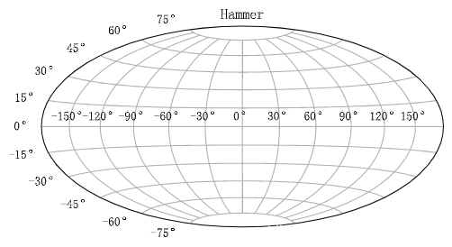
Hammer The mapping procedure is as follows ：

plt.figure()
plt.subplot(projection="hammer")
plt.title("Hammer")
plt.grid(True)

Hammer The result is as follows ：

Lambert The mapping procedure is as follows ：

plt.figure()
plt.subplot(projection="lambert")
plt.title("Lambert")
plt.grid(True)

Lambert The result is as follows ：

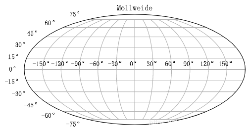
Mollweide The mapping procedure is as follows ：

plt.figure()
plt.subplot(projection="mollweide")
plt.title("Mollweide")
plt.grid(True)

Mollweide The result is as follows ：

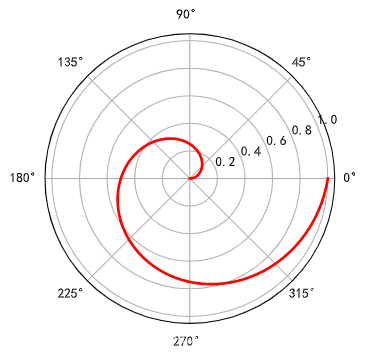
Finally, the most commonly used mapping is introduced polar mapping , That is, the polar coordinate system ,polar The mapping procedure is as follows ：

radi = np.linspace(0, 1, 100)
theta = 2*np.pi*radi

ax = plt.subplot(111, polar=True)
ax.plot(theta, radi, color='r', lw=2)
plt.show()

polar The result is as follows ：

3.3.2 Comprehensive examples

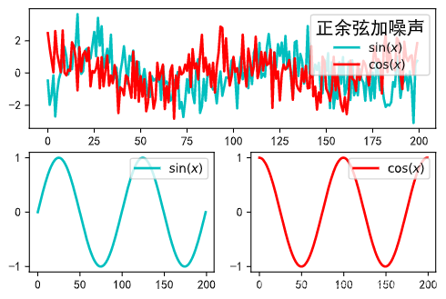
ax = plt.subplot(2, 2, (1, 2))
ax.plot(y+np.random.randn(200), ls='-', lw=2, color='c', label=r'$\sin(x)$')
ax.plot(y1+np.random.randn(200), ls='-', lw=2, color='r', label=r'$\cos(x)$')
ax.legend(title=' Sine and cosine plus noise ', title_fontsize=15, loc='upper right')

ax = plt.subplot(2, 2, 3)
ax.plot(y, ls='-', lw=2, color='c', label=r'$\sin(x)$')
ax.legend(loc='upper right')

ax = plt.subplot(2, 2, 4)
ax.plot(y1, ls='-', lw=2, color='r', label=r'$\cos(x)$')
ax.legend(loc='upper right')

plt.show()

The drawing results are as follows ：

---

Four .add_subplots function

The method is Figure The class method of class is also the most important internal implementation function of the above two functions .

4.1 Function definition

add_subplot(nrows, ncols, index, **kwargs)
           add_subplot(pos, **kwargs)
           add_subplot(ax)
           add_subplot()

add_subplots The parameters of the function are the same as plt.subplot The parameters of the method are almost the same , I won't repeat it again , You can see the above plt.subplot Function introduction .

4.2 Function explanation

The biggest feature of this method is that it is used as a class method , Its use must have corresponding examples , Instead of using... Like the other two functions gcf() Method calls the current Figure object , That means we can work in multiple Figure Object , Accurately create sub graphs on different objects .

4.3 Example of function

4.3.1 Comprehensive examples

The program shows how to accurately create two Figure Partition on object , The example program is as follows ：

import matplotlib.pyplot as plt
import numpy as np
import matplotlib as mpl


mpl.rcParams['font.sans-serif'] = ['SimHei']
mpl.rcParams['axes.unicode_minus'] = False

fig1 = plt.figure(num=1)
fig2 = plt.figure(num=2)
x = np.linspace(-2*np.pi, 2*np.pi, 200)
y = np.sin(x)
y1 = np.cos(x)

ax = fig1.add_subplot(2, 2, (1, 2))
ax.plot(y+np.random.randn(200), ls='-', lw=2, color='c', label=r'$\sin(x)$')
ax.plot(y1+np.random.randn(200), ls='-', lw=2, color='r', label=r'$\cos(x)$')
ax.legend(title=' Sine and cosine plus noise ', title_fontsize=15, loc='upper right')

ax = fig1.add_subplot(2, 2, 3)
ax.plot(y, ls='-', lw=2, color='c', label=r'$\sin(x)$')
ax.legend(loc='upper right')

ax = fig1.add_subplot(2, 2, 4)
ax.plot(y1, ls='-', lw=2, color='r', label=r'$\cos(x)$')
ax.legend(loc='upper right')


x = np.linspace(0, 2 * np.pi, 500)
y = np.sin(x)*np.exp(-x)

ax = fig2.add_subplot(1, 2, 1, title=' Subgraphs 1')
ax.plot(x, y, 'k--', lw=2)
ax.set_title(' Broken line diagram ')

ax = fig2.add_subplot(1, 2, 2, title=' Subgraphs 2')
ax.scatter(x, y, s=10, c='skyblue', marker='o')
ax.set_title(' Scatter plot ')

fig2.subplots_adjust(top=0.8)

plt.show()

The drawing results are as follows ：

---

5、 ... and . summary

Personally, I think the most commonly used must be add_subplot Methods and plt.subplots Method , In general, creating sub areas will not use plt.subplot Method , Its use is to search, not to create . Suppose you need precise control over how to create subareas Figure object , Then use add_subplot Method to create , Usually, if you study or simply draw, you should consider using it directly plt.subplots Method .

---

6、 ... and . Reference resources

1. Visualization solutions
2. The road to Visualization

---