当前位置:网站首页>【深度学习】基于卷积神经网络的天气识别训练
【深度学习】基于卷积神经网络的天气识别训练
2022-08-11 03:53:00 【林夕07】
活动地址:CSDN21天学习挑战赛
目录
前言
关于环境这里不再赘述,与【深度学习】从LeNet-5识别手写数字入门深度学习一文的环境一致。然后需要补充一个pillow包版本7.20即可。
了解weather_photos数据集
该数据包含多云、下雨、晴、日出四种类型天气的照片。分为四个文件夹,每个文件夹对应着该类型的天气图片。
| 文件夹名称 | 天气类型 | 数据量 |
|---|---|---|
| cloudy | 多云 | 300 |
| rain | 下雨 | 215 |
| shine | 晴 | 253 |
| sunrise | 日出 | 357 |
可以看到每种类型的数量不一致,这会影响我们的训练结果。因为下雨的数据集较少,可能会导致识别下雨类型的图片正确率下降等问题。
下载weather_photos数据集
1、可以私信我发你
2、我把数据集打包放在csdn上面,由于最低设置1的币,没有币的同学请私聊我发你就好。下载地址
采用CPU训练还是GPU训练
一般来说有好的显卡(GPU)就使用GPU训练因为快,那么对应的你就要下载tensorflow-gpu包。如果你的显卡较差或者没有足够资金入手一款好的显卡就可以使用CUP训练。
区别
(1)CPU主要用于串行运算;而GPU则是大规模并行运算。由于深度学习中样本量巨大,参数量也很大,所以GPU的作用就是加速网络运算。
(2)CPU计算神经网络也是可以的,算出来的神经网络放到实际应用中效果也很好,只不过速度会很慢罢了。而目前GPU运算主要集中在矩阵乘法和卷积上,其他的逻辑运算速度并没有CPU快。
使用CPU训练
# 使用cpu训练
import os

os.environ["CUDA_VISIBLE_DEVICES"] = "-1"
使用CPU训练时不会显示CPU型号。
使用GPU训练
gpus = tf.config.list_physical_devices("GPU")

if gpus:
    gpu0 = gpus[0]  # 如果有多个GPU,仅使用第0个GPU
    tf.config.experimental.set_memory_growth(gpu0, True)  # 设置GPU显存用量按需使用
    tf.config.set_visible_devices([gpu0], "GPU")
使用GPU训练时会显示对应的GPU型号。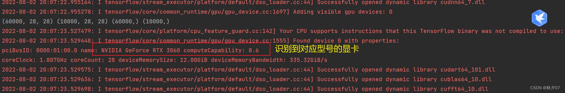
导入数据
这里将本地存放数据集的路径给到data_dir变量中。
import matplotlib.pyplot as plt
import PIL

# 设置随机种子尽可能使结果可以重现
import numpy as np

np.random.seed(1)

# 设置随机种子尽可能使结果可以重现
tf.random.set_seed(1)

from tensorflow import keras
from tensorflow.keras import layers, models

import pathlib

data_dir = "E:\\PythonProject\\day4\\datasets\\weather_photos\\"

data_dir = pathlib.Path(data_dir)
查看数据量
image_count = len(list(data_dir.glob('*/*.jpg')))
print("图片总数为:", image_count)
预处理
加载数据集
这里我们设置了单次训练所抓取的数据样本数量以及图片尺寸。
batch_size = 32
img_height = 180
img_width = 180
并通过image_dataset_from_directory方法将数据集加载到tf.data.dataset中
train_ds = tf.keras.preprocessing.image_dataset_from_directory(
    data_dir,
    validation_split=0.2,
    subset="training",
    seed=123,
    image_size=(img_height, img_width),
    batch_size=batch_size)
加载成功后,会把加载的数据集量以及数据种类打印出来。训练数据集按照80%的量分类并将训练集返回出来。
val_ds = tf.keras.preprocessing.image_dataset_from_directory(
    data_dir,
    validation_split=0.2,
    subset="validation",
    seed=123,
    image_size=(img_height, img_width),
    batch_size=batch_size)
使用同样的方法将测试数据集返回出来,要主要这里的参数只有subset不同。
打印各类型
可以通过class_names方法将数据集的种类进行打印,默认按照文件字母排序
class_names = train_ds.class_names
print(class_names)
运行结果
显示部分图片
首先需要建立一个标签数组,然后绘制前20张,每行5个共四行
from matplotlib import pyplot as plt

plt.figure(figsize=(20, 10))

for images, labels in train_ds.take(1):
    for i in range(20):
        ax = plt.subplot(4, 5, i + 1)

        plt.imshow(images[i].numpy().astype("uint8"))
        plt.title(class_names[labels[i]])

        plt.axis("off")
plt.show()
绘制结果:
配置数据集(加快速度)
shuffle():该函数是将列表的所有元素随机排序。 有时候我们的任务中会使用到随机sample一个数据集的某些数,比如一个文本中,有10行,我们需要随机选取前5个。prefetch():prefetch是预取内存的内容,程序员告诉CPU哪些内容可能马上用到,CPU预取,用于优化。
AUTOTUNE = tf.data.AUTOTUNE

train_ds = train_ds.cache().shuffle(1000).prefetch(buffer_size=AUTOTUNE)
val_ds = val_ds.cache().prefetch(buffer_size=AUTOTUNE)
建立CNN模型
这里新增了一个dropout层。dropout是指在深度学习网络的训练过程中,对于神经网络单元,按照一定的概率将其暂时从网络中丢弃。注意是暂时,对于随机梯度下降来说,由于是随机丢弃,故而每一个mini-batch都在训练不同的网络,防止过拟合。
num_classes = 4
layers.Dropout(0.4)

model = models.Sequential([
    layers.experimental.preprocessing.Rescaling(1./255, input_shape=(img_height, img_width, 3)),

    layers.Conv2D(16, (3, 3), activation='relu', input_shape=(img_height, img_width, 3)),
    layers.AveragePooling2D((2, 2)),
    layers.Conv2D(32, (3, 3), activation='relu'),
    layers.AveragePooling2D((2, 2)),
    layers.Conv2D(64, (3, 3), activation='relu'),
    layers.Dropout(0.3),

    layers.Flatten(),
    layers.Dense(128, activation='relu'),
    layers.Dense(num_classes)
])

model.summary()  # 打印网络结构
网络结构
包含输入层的话总共10层。其中有三个卷积层,俩个最大池化层,一个flatten层,俩个全连接层,一个dropout层。
参数量
总共参数为13M,参数量更加庞大但是数据集不是很多问题不大。建议采用GPU训练。
Total params: 13,794,980
Trainable params: 13,794,980
Non-trainable params: 0
训练模型
训练模型,进行10轮,
# 设置优化器
opt = tf.keras.optimizers.Adam(learning_rate=0.001)

model.compile(optimizer=opt,
              loss=tf.keras.losses.SparseCategoricalCrossentropy(from_logits=True),
              metrics=['accuracy'])

epochs = 10

history = model.fit(
    train_ds,
    validation_data=val_ds,
    epochs=epochs
)
训练结果:测试集acc为87.56%。从效果来说该模型还是不错的。
模型评估
对训练完模型的数据制作成曲线表,方便之后对模型的优化,看是过拟合还是欠拟合还是需要扩充数据等等。
acc = history.history['accuracy']
val_acc = history.history['val_accuracy']

loss = history.history['loss']
val_loss = history.history['val_loss']

epochs_range = range(epochs)

plt.figure(figsize=(12, 4))
plt.subplot(1, 2, 1)
plt.plot(epochs_range, acc, label='Training Accuracy')
plt.plot(epochs_range, val_acc, label='Validation Accuracy')
plt.legend(loc='lower right')
plt.title('Training and Validation Accuracy')

plt.subplot(1, 2, 2)
plt.plot(epochs_range, loss, label='Training Loss')
plt.plot(epochs_range, val_loss, label='Validation Loss')
plt.legend(loc='upper right')
plt.title('Training and Validation Loss')
plt.show()
运行结果:
附录(Anaconda 配置)
将下面的内容进行保存为*.yaml文件即可通过Anaconda软件进行配置导入。
首行的name可以自己修改就是虚拟环境的名称。
name: day5
channels:
  - defaults
dependencies:
  - blas=1.0=mkl
  - ca-certificates=2022.07.19=haa95532_0
  - certifi=2022.6.15=py37haa95532_0
  - cudatoolkit=10.1.243=h74a9793_0
  - cudnn=7.6.5=cuda10.1_0
  - cycler=0.11.0=pyhd3eb1b0_0
  - freetype=2.10.4=hd328e21_0
  - glib=2.69.1=h5dc1a3c_1
  - gst-plugins-base=1.18.5=h9e645db_0
  - gstreamer=1.18.5=hd78058f_0
  - icu=58.2=ha925a31_3
  - intel-openmp=2021.4.0=haa95532_3556
  - jpeg=9e=h2bbff1b_0
  - kiwisolver=1.4.2=py37hd77b12b_0
  - libffi=3.4.2=hd77b12b_4
  - libiconv=1.16=h2bbff1b_2
  - libogg=1.3.5=h2bbff1b_1
  - libpng=1.6.37=h2a8f88b_0
  - libtiff=4.2.0=he0120a3_1
  - libvorbis=1.3.7=he774522_0
  - libwebp=1.2.2=h2bbff1b_0
  - libxml2=2.9.14=h0ad7f3c_0
  - libxslt=1.1.35=h2bbff1b_0
  - lz4-c=1.9.3=h2bbff1b_1
  - matplotlib=3.2.1=0
  - matplotlib-base=3.2.1=py37h64f37c6_0
  - mkl=2021.4.0=haa95532_640
  - mkl-service=2.4.0=py37h2bbff1b_0
  - mkl_fft=1.3.1=py37h277e83a_0
  - mkl_random=1.2.2=py37hf11a4ad_0
  - numpy-base=1.21.5=py37hca35cd5_3
  - olefile=0.46=py37_0
  - openssl=1.1.1q=h2bbff1b_0
  - packaging=21.3=pyhd3eb1b0_0
  - pcre=8.45=hd77b12b_0
  - pillow=8.0.0=py37hca74424_0
  - pip=22.1.2=py37haa95532_0
  - ply=3.11=py37_0
  - pyparsing=3.0.4=pyhd3eb1b0_0
  - pyqt=5.15.7=py37hd77b12b_0
  - pyqt5-sip=12.11.0=py37hd77b12b_0
  - python=3.7.0=hea74fb7_0
  - python-dateutil=2.8.2=pyhd3eb1b0_0
  - qt-main=5.15.2=he8e5bd7_4
  - qt-webengine=5.15.9=hb9a9bb5_4
  - qtwebkit=5.212=h3ad3cdb_4
  - setuptools=61.2.0=py37haa95532_0
  - sip=6.6.2=py37hd77b12b_0
  - six=1.16.0=pyhd3eb1b0_1
  - sqlite=3.38.5=h2bbff1b_0
  - tk=8.6.12=h2bbff1b_0
  - toml=0.10.2=pyhd3eb1b0_0
  - tornado=6.1=py37h2bbff1b_0
  - typing_extensions=4.1.1=pyh06a4308_0
  - vc=14.2=h21ff451_1
  - vs2015_runtime=14.27.29016=h5e58377_2
  - wheel=0.37.1=pyhd3eb1b0_0
  - wincertstore=0.2=py37haa95532_2
  - xz=5.2.5=h8cc25b3_1
  - zlib=1.2.12=h8cc25b3_2
  - zstd=1.5.2=h19a0ad4_0
  - pip:
    - absl-py==1.2.0
    - astor==0.8.1
    - astunparse==1.6.3
    - cachetools==4.2.4
    - charset-normalizer==2.1.0
    - flatbuffers==2.0
    - gast==0.2.2
    - google-auth==1.35.0
    - google-auth-oauthlib==0.4.6
    - google-pasta==0.2.0
    - grpcio==1.48.0
    - h5py==3.7.0
    - idna==3.3
    - importlib-metadata==4.12.0
    - keras-applications==1.0.8
    - keras-nightly==2.11.0.dev2022080907
    - keras-preprocessing==1.1.2
    - libclang==14.0.6
    - markdown==3.4.1
    - markupsafe==2.1.1
    - numpy==1.21.6
    - oauthlib==3.2.0
    - opt-einsum==3.3.0
    - protobuf==3.19.4
    - pyasn1==0.4.8
    - pyasn1-modules==0.2.8
    - requests==2.28.1
    - requests-oauthlib==1.3.1
    - rsa==4.9
    - scipy==1.4.1
    - tb-nightly==2.10.0a20220809
    - tensorboard==2.1.1
    - tensorboard-data-server==0.6.1
    - tensorboard-plugin-wit==1.8.1
    - tensorflow==2.1.0
    - tensorflow-estimator==2.1.0
    - tensorflow-io-gcs-filesystem==0.26.0
    - termcolor==1.1.0
    - tf-estimator-nightly==2.11.0.dev2022080908
    - tf-nightly==2.11.0.dev20220808
    - typing-extensions==4.3.0
    - urllib3==1.26.11
    - werkzeug==2.2.1
    - wrapt==1.14.1
    - zipp==3.8.1
边栏推荐
- js uses the string as the js execution code
- watch监听
- 80端口和443端口是什么?有什么区别?
- 移动端地图开发选择哪家?
- Binary tree related code questions [more complete] C language
- How to rebuild after pathman_config and pathman_config_params are deleted?
- Design and Realization of Employment Management System in Colleges and Universities
- Will oracle cardinality affect query speed?
- 机器学习中什么是集成学习?
- es-head plugin insert query and conditional query (5)
猜你喜欢
![[FPGA] day19- binary to decimal (BCD code)](/img/d8/6d223e5e81786335a143f135385b08.png)
[FPGA] day19- binary to decimal (BCD code)

Homework 8.10 TFTP protocol download function

Rotary array problem: how to realize the array "overall reverse, internal orderly"?"Three-step conversion method" wonderful array

EasyCVR接入海康大华设备选择其它集群服务器时,通道ServerID错误该如何解决?

多串口RS485工业网关BL110

【FPGA】abbreviation
高校就业管理系统设计与实现

【FPGA】day20-I2C读写EEPROM

LeetCode刷题第16天之《239滑动窗口最大值》

Which one to choose for mobile map development?
随机推荐
"98 BST and Its Verification" of the 13th day of leetcode brushing series of binary tree series
MySQL数据库存储引擎以及数据库的创建、修改与删除
80端口和443端口是什么?有什么区别?
元素的BFC属性
E-commerce project - mall time-limited seckill function system
Is Redis old?Performance comparison between Redis and Dragonfly
论文精度 —— 2017 CVPR《High-Resolution Image Inpainting using Multi-Scale Neural Patch Synthesis》
Multi-merchant mall system function disassembly 26 lectures - platform-side distribution settings
Enter the starting position, the ending position intercepts the linked list
Which one to choose for mobile map development?
The impact of programmatic trading and subjective trading on the profit curve!
程序化交易的策略类型可以分为哪几种?
STC8H开发(十五): GPIO驱动Ci24R1无线模块
LeetCode刷题第12天二叉树系列之《104 二叉树的最大深度》
荣威imax8ev魔方电池安全感,背后隐藏着哪些黑化膨胀?
Use jackson to parse json data in detail
这些云自动化测试工具值得拥有
Read the article, high-performance and predictable data center network
拼多多店铺营业执照相关问题
Is there any way for kingbaseES to not read the system view under sys_catalog by default?