Convolution of images

Quotation translation ：《 Hands-on deep learning 》

Now we have seen how the convolution layer works in theory , We're going to see how this works in practice . Because we motivate it through the applicability of convolutional neural network to image data , We will insist on using image data in our example , And start revisiting the convolution layer we introduced in the previous section . We noticed that , Strictly speaking , Convolution layer is a slight misnomer , Because operations are usually represented as cross associations .

One 、 Cross correlation operation

In the accretion layer , An input array and a related kernel array are combined , Generate an output array through cross correlation operation . Let's see how this works in two-dimensional space . In our case , The input is a height of 3, Width is 3 Two dimensional array of , We mark the shape of the array as 3×3 or （3,3）. The height and width of the core array are 2. In the field of deep learning research , Common names for this array include kernel and filter . Kernel window （ Also known as convolution window ） The shape of the core is precisely given by the height and width of the core （ Here is 2×2）.

​

​

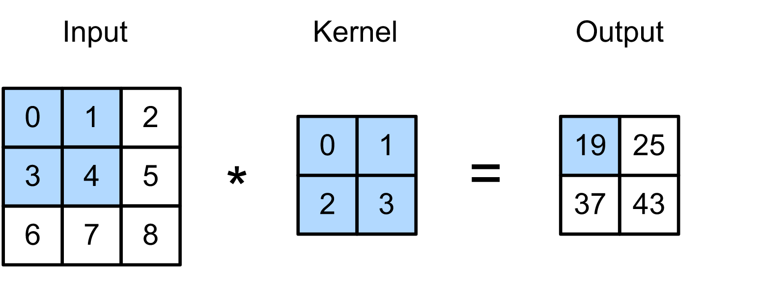
chart ： Two dimensional cross correlation operation . The shaded part is the first output element and the input and kernel array elements used for its calculation . 0×0+1×1+3×2+4×3=19 .

In two-dimensional cross-correlation operation , Let's start with the convolution window in the upper left corner of the input array , Then slide on the input array from left to right and from top to bottom . When the convolution window slides to a certain position , The input subarray contained in this window is multiplied by the kernel array （ In terms of elements ）, The resulting arrays are added to produce a single scalar value . The result is the value of the output array at the corresponding position . here , The height of the output array is 2, Width is 2, The four elements come from two-dimensional cross-correlation operations .

Please note that , Along each axis , The output is slightly smaller than the input . Because the width of the kernel is larger than 1, Moreover, we can only calculate the cross-correlation of the position where the kernel is completely suitable for the image , The output size is determined by the input size 𝐻×𝑊 Subtract the size of the convolution kernel ℎ×𝑤, namely （𝐻-ℎ+1）×（𝑊-𝑤+1） give . This is because we need enough space on the image " Move " Convolution kernel （ Later we'll see how to keep the size constant by filling zero around the image boundary , So there is enough space to move the core ）. Next , We are corr2d Function to implement the above process . It accepts arrays with kernels K Input array of X, And output the array Y.

import torch
from torch import nn

def corr2d(X, K):
    h, w = K.shape  #  The size of the convolution kernel 
    print('h,w: ',h,w)
    Y = torch.zeros((X.shape[0] - h + 1, X.shape[1] - w + 1))
    for i in range(Y.shape[0]):
        for j in range(Y.shape[1]):
            Y[i, j] = (X[i: i + h, j: j + w] * K).sum()  #  Add after dot multiplication 
    return Y

We can build the input array from the above figure X And kernel array K To verify the output of the implementation of the above two-dimensional cross-correlation operation .

X = torch.Tensor([[0, 1, 2], [3, 4, 5], [6, 7, 8]])
K = torch.Tensor([[0, 1], [2, 3]])
Y = corr2d(X, K)
print('Y: ' ,Y)

h,w:   2 2
 The convolution part   : tensor([[0., 1.],
        [3., 4.]])
 The convolution part   : tensor([[1., 2.],
        [4., 5.]])
 The convolution part   : tensor([[3., 4.],
        [6., 7.]])
 The convolution part   : tensor([[4., 5.],
        [7., 8.]])
Y:  tensor([[19., 25.],
        [37., 43.]])

Two 、 Convolution layer

The convolution layer cross correlates the input and kernel , And add a scalar offset to produce an output . The parameters of the convolution layer are The values that make up the kernel and scalar offsets . When training a convolution based model , We usually initialize the kernel randomly , Just like we do for the full connection layer .

We are now ready to define the above corr2d Function to realize a two-dimensional convolution layer .

stay __init__ In the constructor , We declare that weight and bias are two model parameters . Forward calculation function forward call corr2d Function and add offset . And ℎ×𝑤 Cross correlation , We also call the convolution layer ℎ×𝑤 Convolution .

class Conv2D(nn.Module):
    def __init__(self, kernel_size, **kwargs):
        super(Conv2D, self).__init__(**kwargs)
        #  Pass in kernel_size Convolution kernel size 
        self.weight = torch.rand(kernel_size,dtype=torch.float32,requires_grad=True)
        self.bias = torch.zeros((1,),dtype=torch.float32,requires_grad=True)

    def forward(self, x):
        
        return corr2d(x, self.weight) + self.bias

3、 ... and 、 Object edge detection in image

Let's look at a simple application of convolution ： The edge of the object in the image is detected by looking for the position of the pixel change . First , Let's build a 6×8 Pixel “ Images ”. The middle four columns are black （0）, The rest is white （1）.

X = torch.ones((6, 8))
X[:, 2:6] = 0
X

tensor([[1., 1., 0., 0., 0., 0., 1., 1.],
        [1., 1., 0., 0., 0., 0., 1., 1.],
        [1., 1., 0., 0., 0., 0., 1., 1.],
        [1., 1., 0., 0., 0., 0., 1., 1.],
        [1., 1., 0., 0., 0., 0., 1., 1.],
        [1., 1., 0., 0., 0., 0., 1., 1.]])

Next , We build a high degree of 1、 Width is 2 The kernel of K. When we cross correlate inputs , If the horizontally adjacent elements are the same , The output of 0, otherwise , The output is non-zero .

K = torch.Tensor([[1, -1]])
print('K: ',K)

K:  tensor([[ 1., -1.]])

Input X And the kernel we designed K To perform cross-correlation operations . As you can see , We will detect that the edge from white to black is 1, The edge from black to white is -1. The rest of the output is 0.

Y = corr2d(X, K)
print('Y: ',Y)

h,w:   1 2
Y:  tensor([[ 0.,  1.,  0.,  0.,  0., -1.,  0.],
        [ 0.,  1.,  0.,  0.,  0., -1.,  0.],
        [ 0.,  1.,  0.,  0.,  0., -1.,  0.],
        [ 0.,  1.,  0.,  0.,  0., -1.,  0.],
        [ 0.,  1.,  0.,  0.,  0., -1.,  0.],
        [ 0.,  1.,  0.,  0.,  0., -1.,  0.]])

Let's apply the kernel to the transposed image . As expected , It's gone . kernel K Detect only vertical edges .

corr2d(X.t(), K)  #  take X Transposition , If the horizontally adjacent elements are the same , The output of 0, otherwise , The output is non-zero . So you can't detect 

h,w:   1 2

tensor([[0., 0., 0., 0., 0.],
        [0., 0., 0., 0., 0.],
        [0., 0., 0., 0., 0.],
        [0., 0., 0., 0., 0.],
        [0., 0., 0., 0., 0.],
        [0., 0., 0., 0., 0.],
        [0., 0., 0., 0., 0.],
        [0., 0., 0., 0., 0.]])

Transpose at the same time X and K, Then the edge appears ：

#  Transpose at the same time X and K, Then the edge appears 
corr2d(X.t(), K.t())

h,w:   2 1





tensor([[ 0.,  0.,  0.,  0.,  0.,  0.],
        [ 1.,  1.,  1.,  1.,  1.,  1.],
        [ 0.,  0.,  0.,  0.,  0.,  0.],
        [ 0.,  0.,  0.,  0.,  0.,  0.],
        [ 0.,  0.,  0.,  0.,  0.,  0.],
        [-1., -1., -1., -1., -1., -1.],
        [ 0.,  0.,  0.,  0.,  0.,  0.]])

Four 、 Learn a kernel

If we know this is what we are looking for , So by finite difference [1, -1] To design an edge detector is very good . However , When we see larger nuclei , And considering the continuous convolution layer , It may not be possible to manually specify exactly what each filter should do .

Now let's see if we can just look at （ Input , Output ） To learn from X Generate Y The kernel of . We first build a convolution layer , And initialize its kernel into a random array . Next , In each iteration , We will use the square error to compare Y And the output of the convolution layer , Then calculate the gradient to update the weight . For the sake of simplicity , In this convolution layer , We will ignore the bias .

We built Conv2D class . But here we use Pytorch In the library nn.Conv2D. The custom class we created Conv2D You can use... Similarly .

#  Build a with 1 Convolution layer of two output channels （ The channel will be introduced in the next section ）, The shape of the kernel array is （1,2）

conv2d = nn.Conv2d(1,1, kernel_size=(1, 2),bias=False) #  For the sake of simplicity , Ignore bias 

#  Two dimensional convolution uses four-dimensional input and output , The format is （ Example channel , Height , Width ）, The batch size （ Number of examples in batch ） And the number of channels is 1
X = X.reshape((1, 1, 6, 8))  #  Previous input X
print('X: ',X)

Y = Y.reshape((1, 1, 6, 7))  #  After a corr2d Output Y（ As a standard label , To learn convolution kernel parameters ）
print('Y: ',Y)

for i in range(10):
    Y_hat = conv2d(X)
    l = (Y_hat - Y) ** 2  #  Defined loss function , Square difference distance 
    conv2d.zero_grad()
    l.sum().backward()  #  Back propagation calculation 
    #  For the sake of simplicity , We ignore the problem of deviation here 
    conv2d.weight.data[:] -= 3e-2 * conv2d.weight.grad  #  Update weights 
    if (i + 1) % 2 == 0:
        print('batch %d, loss %.3f' % (i + 1, l.sum()))  #  Output 

X:  tensor([[[[1., 1., 0., 0., 0., 0., 1., 1.],
          [1., 1., 0., 0., 0., 0., 1., 1.],
          [1., 1., 0., 0., 0., 0., 1., 1.],
          [1., 1., 0., 0., 0., 0., 1., 1.],
          [1., 1., 0., 0., 0., 0., 1., 1.],
          [1., 1., 0., 0., 0., 0., 1., 1.]]]])
Y:  tensor([[[[ 0.,  1.,  0.,  0.,  0., -1.,  0.],
          [ 0.,  1.,  0.,  0.,  0., -1.,  0.],
          [ 0.,  1.,  0.,  0.,  0., -1.,  0.],
          [ 0.,  1.,  0.,  0.,  0., -1.,  0.],
          [ 0.,  1.,  0.,  0.,  0., -1.,  0.],
          [ 0.,  1.,  0.,  0.,  0., -1.,  0.]]]])
batch 2, loss 3.774
batch 4, loss 0.676
batch 6, loss 0.131
batch 8, loss 0.029
batch 10, loss 0.008

As you can see , stay 10 After iterations , The error has dropped to a very small value . Now let's take a look at what we learned about kernel arrays .

conv2d.weight.data.reshape((1, 2))

tensor([[ 1.0121, -0.9671]])

When considering bias ：

#  Constructing a kernel array shape is (1, 2) Two dimensional convolution 
conv2d = Conv2D(kernel_size=(1, 2))

step = 20
lr = 0.01
for i in range(step):
    Y_hat = conv2d(X)
    l = ((Y_hat - Y) ** 2).sum()
    l.backward()

    #  gradient descent 
    conv2d.weight.data -= lr * conv2d.weight.grad
    conv2d.bias.data -= lr * conv2d.bias.grad

    #  Gradient clear 0
    conv2d.weight.grad.fill_(0)
    conv2d.bias.grad.fill_(0)
    if (i + 1) % 5 == 0:
        print('Step %d, loss %.3f' % (i + 1, l.item()))

h,w:   1 2
h,w:   1 2
h,w:   1 2
h,w:   1 2
h,w:   1 2
Step 5, loss 5.881
h,w:   1 2
h,w:   1 2
h,w:   1 2
h,w:   1 2
h,w:   1 2
Step 10, loss 1.410
h,w:   1 2
h,w:   1 2
h,w:   1 2
h,w:   1 2
h,w:   1 2
Step 15, loss 0.367
h,w:   1 2
h,w:   1 2
h,w:   1 2
h,w:   1 2
h,w:   1 2
Step 20, loss 0.099

#  Output results 
print("weight: ", conv2d.weight.data)
print("bias: ", conv2d.bias.data)

weight:  tensor([[ 0.9268, -0.9145]])
bias:  tensor([-0.0069])

in fact , The learned kernel array is different from the kernel array we defined before K Very close to .

5、 ... and 、 Cross correlation and convolution

actually , Convolution is similar to cross-correlation . In order to get the output of convolution , We just flip the core array left and right and up and down , Then do cross-correlation operation with the input array . so , Convolution and cross-correlation are similar , But if they use the same core array , For the same input , The output is often different .

that , You may wonder why convolution can be replaced by cross-correlation in convolution . Actually , In deep learning, kernel arrays are learned ： Whether the convolution layer uses cross-correlation operation or convolution operation, it does not affect the output of model prediction . To explain this . In order to be consistent with most in-depth learning literature , If there is no special instruction , The convolution operation mentioned in this book refers to cross-correlation operation .

6、 ... and 、 summary

The core calculation of two-dimensional convolution is a two-dimensional cross-correlation operation . In its simplest form , It performs cross-correlation operation between two-dimensional input data and kernel , Then add an offset .
We can design a kernel to detect the edge in the image .
We can learn the kernel from the data .

7、 ... and 、 practice

1、 Build an image with diagonal edges X.

• If you apply the kernel to it K, What's going to happen ？
• If you will X Transposition , What's going to happen ？
• If you transpose K What's going to happen ？

① Constructing diagonal image matrix

#  Constructing diagonal image matrix 
Z = torch.ones((8, 8))
for i in range(len(Z)):
    Z[i, i] = 0
print('Z:',Z)

Z: tensor([[0., 1., 1., 1., 1., 1., 1., 1.],
        [1., 0., 1., 1., 1., 1., 1., 1.],
        [1., 1., 0., 1., 1., 1., 1., 1.],
        [1., 1., 1., 0., 1., 1., 1., 1.],
        [1., 1., 1., 1., 0., 1., 1., 1.],
        [1., 1., 1., 1., 1., 0., 1., 1.],
        [1., 1., 1., 1., 1., 1., 0., 1.],
        [1., 1., 1., 1., 1., 1., 1., 0.]])

② Apply convolution kernel K To deal with Z

#  Apply convolution kernel K To deal with Z
corr2d(Z, K)

h,w:   1 2

tensor([[-1.,  0.,  0.,  0.,  0.,  0.,  0.],
        [ 1., -1.,  0.,  0.,  0.,  0.,  0.],
        [ 0.,  1., -1.,  0.,  0.,  0.,  0.],
        [ 0.,  0.,  1., -1.,  0.,  0.,  0.],
        [ 0.,  0.,  0.,  1., -1.,  0.,  0.],
        [ 0.,  0.,  0.,  0.,  1., -1.,  0.],
        [ 0.,  0.,  0.,  0.,  0.,  1., -1.],
        [ 0.,  0.,  0.,  0.,  0.,  0.,  1.]])

③ If you will Z Transposition , What's going to happen

#  If you will Z Transposition , What's going to happen 
corr2d(Z.t(), K)
#  unchanged 

h,w:   1 2

Output ：

tensor([[-1.,  0.,  0.,  0.,  0.,  0.,  0.],
        [ 1., -1.,  0.,  0.,  0.,  0.,  0.],
        [ 0.,  1., -1.,  0.,  0.,  0.,  0.],
        [ 0.,  0.,  1., -1.,  0.,  0.,  0.],
        [ 0.,  0.,  0.,  1., -1.,  0.,  0.],
        [ 0.,  0.,  0.,  0.,  1., -1.,  0.],
        [ 0.,  0.,  0.,  0.,  0.,  1., -1.],
        [ 0.,  0.,  0.,  0.,  0.,  0.,  1.]])

④ Transposition K What's going to happen ？

#  If you transpose K What's going to happen ？
corr2d(Z, K.t())

#  The secondary diagonal will change above 

h,w:   2 1

tensor([[-1.,  1.,  0.,  0.,  0.,  0.,  0.,  0.],
        [ 0., -1.,  1.,  0.,  0.,  0.,  0.,  0.],
        [ 0.,  0., -1.,  1.,  0.,  0.,  0.,  0.],
        [ 0.,  0.,  0., -1.,  1.,  0.,  0.,  0.],
        [ 0.,  0.,  0.,  0., -1.,  1.,  0.,  0.],
        [ 0.,  0.,  0.,  0.,  0., -1.,  1.,  0.],
        [ 0.,  0.,  0.,  0.,  0.,  0., -1.,  1.]])

2、 How do you change the input and kernel array to represent a cross-correlation operation, matrix multiplication ？

Why should convolution be transformed into matrix multiplication ？

To speed up the operation , The traditional calculation method of convolution kernel sliding in turn is difficult to accelerate .

After converting to matrix multiplication , You can call various linear algebra operation Libraries ,CUDA Inside the matrix multiplication implementation . These matrix multiplications are limit optimized , Many times faster than violent calculation .

3、 Manually design some kernels .

• What is the form of the kernel of the second derivative ？
• What is the kernel of Laplacian ？
• What is the kernel of integral ？
• In order to get a degree of 𝑑 The derivative of , What is the minimum size of the kernel ？