logistic Return chapter

The data set corresponds to the data set in the previous section , This analysis is based on whether users are high response users , Use logistic Regression is used to predict the responsiveness of users , The probability of getting a response . Linear regression , Refer to the previous chapter

1 Read and preview data

Load and read the data , The data is still desensitized data ,

file_path<-"data_response_model.csv" #change the location

# read in data
options(stringsAsFactors = F)
raw<-read.csv(file_path)   #read in your csv data
str(raw)     #check the varibale type
View(raw)    #take a quick look at the data
summary(raw) #take a quick look at the summary of variable

# response variable
View(table(raw$dv_response))  #Y
View(prop.table(table(raw$dv_response))) #Y frequency

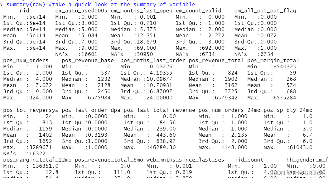
Determine according to the business , Data y The value is the response rate is dv_response, And observe the situation

2 Divide the data

Still divide the data into three parts , They are training sets , Validation set and test set .

#Separate Build Sample
train<-raw[raw$segment=='build',]  #select build sample, it should be random selected when you build the model
View(table(train$segment))         #check segment
View(table(train$dv_response))     #check Y distribution  
View(prop.table(table(train$dv_response))) #check Y distribution

#Separate invalidation Sample
test<-raw[raw$segment=='inval',] #select invalidation(OOS) sample
View(table(test$segment))       #check segment
View(prop.table(table(test$dv_response))) #check Y distribution

#Separate out of validation Sample
validation<-raw[raw$segment=='outval',] #select out of validation(OOT) sample
View(table(validation$segment)) #check segment
View(prop.table(table(validation$dv_response))) #check Y distribution

3 profilng Make

Sum the response rates in the data , The high response customers in the original data are 1, Low response customers are 0. The total number of summations is the number of highly responsive customers ,length Is the total number of records , The average is the overall average

# overall performance
overall_cnt=nrow(train)   #calculate the total count
overall_resp=sum(train$dv_response)  #calculate the total responders count
overall_resp_rate=overall_resp/overall_cnt  #calculate the response rate
overall_perf<-c(overall_count=overall_cnt,overall_responders=overall_resp,overall_response_rate=overall_resp_rate) #combine
overall_perf<-c(overall_cnt=nrow(train),overall_resp=sum(train$dv_response),overall_resp_rate=sum(train$dv_response)/nrow(train)) #combine
View(t(overall_perf))  #take a look at the summary

The division here is the same as that in the previous chapter lift Picture making , Also available sql To write , Like group by, Calculate the comparison between the average response rate of each group and the overall response rate .
stay library Before , Please download first plyr package , Write sql Need to download sqldf
install.packages(“sqldf”)

library(plyr)              #call plyr
?ddply
prof<-ddply(train,.(hh_gender_m_flag),summarise,cnt=length(rid),res=sum(dv_response)) #group by hh_gender_m_flg
View(prof)  #check the result
tt=aggregate(train[,c("hh_gender_m_flag","rid")],by=list(train[,c("hh_gender_m_flag")]),length) #group by hh_gender_m_flg
View(tt) 
#calculate the probablity
#prop.table(as.matrix(prof[,-1]),2)
#t(t(prof)/colSums(prof))

prof1<-within(prof,{res_rate<-res/cnt 
index<-res_rate/overall_resp_rate*100
percent<-cnt/overall_cnt
})  #add response_rate,index, percentage

View(prof1)   #check the result

library(sqldf)
# Integer multiply floating point variable floating point data
sqldf("select hh_gender_m_flag,count() as cnt,sum(dv_response)as res,1.0sum(dv_response) /count(*) as res_rate from train group by 1 ")
Missing values can also be part of a feature , Missing values can also be lift Compare

nomissing<-data.frame(var_data[!is.na(var_data$em_months_last_open),])  #select the no missing value records 
missing<-data.frame(var_data[is.na(var_data$em_months_last_open),])     #select the missing value records

###################################### numeric Profiling:missing part   #############################################################

missing2<-ddply(missing,.(em_months_last_open),summarise,cnt=length(dv_response),res=sum(dv_response)) #group by em_months_last_open
View(missing2)  

missing_perf<-within(missing2,{res_rate<-res/cnt 
index<-res_rate/overall_resp_rate*100
percent<-cnt/overall_cnt
var_category<-c('unknown')
})   #summary

View(missing_perf)

Here, the non missing value data are divided , Add non missing value data , It is divided into 10 Equal division . Calculate the total number of records and the total number of highly responsive customers respectively

nomissing_value<-nomissing$em_months_last_open  #put the nomissing values into a variable

#method1:equal frequency
nomissing$var_category<-cut(nomissing_value,unique(quantile(nomissing_value,(0:10)/10)),include.lowest = T)#separte into 10 groups based on records
class(nomissing$var_category)
View(table(nomissing$var_category))  #take a look at the 10 category

prof2<-ddply(nomissing,.(var_category),summarise,cnt=length(dv_response),res=sum(dv_response)) #group by the 10 groups
View(prof2)

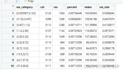
Divide the into 10 Each group of equally divided data is lift Calculation , Compare the ratio of the average number of high response applications in each group to the total number of users . Greater than 100% Is the customer label higher than the overall performance

nonmissing_perf<-within(prof2,
                        {res_rate<-res/cnt 
                        index<-res_rate/overall_resp_rate*100
                        percent<-cnt/overall_cnt
                        })  #add resp_rate,index,percent
View(nonmissing_perf)

#set missing_perf and non-missing_Perf together
View(missing_perf)
View(nonmissing_perf)
em_months_last_open_perf<-rbind(nonmissing_perf,missing_perf[,-1]) #set 2 data together
View(em_months_last_open_perf)

4 Missing value , Exception handling

1 Less than 3% Directly delete or median , Average fill
2 3%——20% Delete or knn,EM Return to fill
3 20%——50% Multiple imputation
4 50——80% Missing value taxonomy
5 higher than 80% discarded , The data is too inaccurate , There are a lot of mistakes in analysis

Outliers are usually solved by capping

numeric variables

train$m2_em_count_valid <- ifelse(is.na(train$em_count_valid) == T, 2,      #when em_count_valid is missing ,then assign 2
                                  ifelse(train$em_count_valid <= 1, 1,         #when em_count_valid<=1 then assign 1
                                         ifelse(train$em_count_valid >=10, 10, #when em_count_valid>=10 then assign 10
                                                train$em_count_valid)))        #when 1<em_count_valid<10 and not missing then assign the raw value

summary(train$m2_em_count_valid)  #do a summary
summary(train$m1_EM_COUNT_VALID)  #do a summary

5 Model fitting

Select the most valuable variables according to the business

library(picante)  #call picante
var_list<-c('dv_response','m1_POS_NUM_ORDERS_24MO',
            'm1_POS_NUM_ORDERS',
            'm1_SH_MNTHS_LAST_INQUIRED',
            'm1_POS_SP_QTY_24MO',
            'm1_POS_REVENUE_TOTAL',
            'm1_POS_LAST_ORDER_DPA',
            'm1_POS_MARGIN_TOTAL',
            'm1_pos_mo_btwn_fst_lst_order',
            'm1_POS_REVENUE_BASE',
            'm1_POS_TOT_REVPERSYS',
            'm1_EM_COUNT_VALID',
            'm1_EM_NUM_OPEN_30',
            'm1_POS_MARGIN_TOTAL_12MO',
            'm1_EX_AUTO_USED0005_X5',
            'm1_SH_INQUIRED_LAST3MO',
            'm1_EX_AUTO_USED0005_X789',
            'm1_HH_INCOME',
            'm1_SH_INQUIRED_LAST12MO',
            'm1_POS_LAST_TOTAL_REVENUE',
            'm1_EM_ALL_OPT_OUT_FLAG',
            'm1_POS_REVENUE_TOTAL_6MO',
            'm1_EM_MONTHS_LAST_OPEN',
            'm1_POS_MNTHS_LAST_ORDER',
            'm1_WEB_MNTHS_SINCE_LAST_SES')  #put the variables you want to do correlation analysis here

Make correlation coefficient matrix , Filter the related variables according to the correlation , Collinearity selection identification variable method or dummy variable method ,logistic Regression can use IV Value selection variable

corr_var<-train[, var_list]  #select all the variables you want to do correlation analysis
str(corr_var)                #check the variable type
correlation<-data.frame(cor.table(corr_var,cor.method = 'pearson'))  #do the correlation
View(correlation)
cor_only=data.frame(row.names(correlation),correlation[, 1:ncol(corr_var)])  #select correlation result only
View(cor_only)

Select the , Variables ready to be put into the model

var_list<-c('m1_WEB_MNTHS_SINCE_LAST_SES',
            'm1_POS_MNTHS_LAST_ORDER',
            'm1_POS_NUM_ORDERS_24MO',
            'm1_pos_mo_btwn_fst_lst_order',
            'm1_EM_COUNT_VALID',
            'm1_POS_TOT_REVPERSYS',
            'm1_EM_MONTHS_LAST_OPEN',
            'm1_POS_LAST_ORDER_DPA'
)   #put the variables you want to try in model here

mods<-train[,c(‘dv_response’,var_list)] #select Y and varibales you want to try
str(mods)
Non standardized fitting , After fitting, stepwise regression was used to screen variables

mods<-train[,c('dv_response',var_list)]  #select Y and varibales you want to try
str(mods)

(model_glm<-glm(dv_response~.,data=mods,family =binomial(link ="logit")))  #logistic model
model_glm
#Stepwise
library(MASS)
model_sel<-stepAIC(model_glm,direction ="both")  #using both backward and forward stepwise selection
model_sel
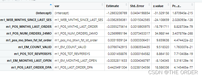
summary<-summary(model_sel)  #summary
model_summary<-data.frame(var=rownames(summary$coefficients),summary$coefficients) #do the model summary
View(model_summary)

Modeling after data standardization , Standardized modeling makes it easy to view each variable pair y The degree of influence

#variable importance
#standardize variable

#?scale
mods2<-scale(train[,var_list],center=T,scale=T) 
mods3<-data.frame(dv_response=c(train$dv_response),mods2[,var_list])
# View(mods3)
(model_glm2<-glm(dv_response~.,data=mods3,family =binomial(link ="logit")))  #logistic model
(summary2<-summary(model_glm2)) 
model_summary2<-data.frame(var=rownames(summary2$coefficients),summary2$coefficients) #do the model summary
View(model_summary2)
model_summary2_f<-model_summary2[model_summary2$var!='(Intercept)',]
model_summary2_f$contribution<-abs(model_summary2_f$Estimate)/(sum(abs(model_summary2_f$Estimate)))
View(model_summary2_f)

6 Model to evaluate

Regression fitting VIF value

#Variable VIF
fit <- lm(dv_response~., data=mods)  #regression model
#install.packages('car')  #Install Package 'Car' to calculate VIF
require(car)  #call Car
vif=data.frame(vif(fit)) #get Vif
var_vif=data.frame(var=rownames(vif),vif) #get variables and corresponding Vif
View(var_vif)

Production of correlation coefficient matrix

#variable correlation
cor<-data.frame(cor.table(mods,cor.method = 'pearson')) #calculate the correlation
correlation<-data.frame(variables=rownames(cor),cor[, 1:ncol(mods)]) #get correlation only
View(correlation)

Finally, make ROC curve , Draw on the model ROC diagram , Observe the effect

library(ROCR)

#### test data####
pred_prob<-predict(model_glm,test,type='response') #predict Y
pred_prob
pred<-prediction(pred_prob,test$dv_response) #put predicted Y and actual Y together
pred@predictions
View(pred)
perf<-performance(pred,'tpr','fpr')   #Check the performance,True positive rate
perf
par(mar=c(5,5,2,2),xaxs = "i",yaxs = "i",cex.axis=1.3,cex.lab=1.4)  #set the graph parameter

#AUC value
auc <- performance(pred,"auc")
unlist(slot(auc,"y.values"))

#plotting the ROC curve
plot(perf,col="black",lty=3, lwd=3,main='ROC Curve')

#plot Lift chart
perf<-performance(pred,‘lift’,‘rpp’)
plot(perf,col=“black”,lty=3, lwd=3,main=‘Lift Chart’)

7 Overall division of user groups lift chart

pred<-predict(model_glm,train,type='response')   #Predict Y
decile<-cut(pred,unique(quantile(pred,(0:10)/10)),labels=10:1, include.lowest = T)  #Separate into 10 groups
sum<-data.frame(actual=train$dv_response,pred=pred,decile=decile) #put actual Y,predicted Y,Decile together

decile_sum<-ddply(sum,.(decile),summarise,cnt=length(actual),res=sum(actual)) #group by decile
decile_sum2<-within(decile_sum,
                     {res_rate<-res/cnt 
                    index<-100*res_rate/(sum(res)/sum(cnt))
                     })  #add resp_rate,index
decile_sum3<-decile_sum2[order(decile_sum2[,1],decreasing=T),] #order decile
View(decile_sum3)

The decile division is adopted , Division of the number of records, customer groups , You can find 1-10 A hierarchy of users , True response rate lift Good value .
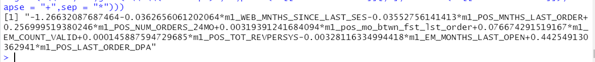
Post the regression equation

ss <- summary(model_glm)  #put model summary together
ss
which(names(ss)=="coefficients")

#XBeta
#Y = 1/(1+exp(-XBeta))
#output model equoation
gsub("\\+-","-",gsub('\\*\\(Intercept)','',paste(ss[["coefficients"]][,1],rownames(ss[["coefficients"]]),collapse = "+",sep = "*")))