Chapter 2 pytoch foundation 2

link

2.5 Tensor And Autograd

In the neural network , An important content is parameter learning , And parameter learning is inseparable from derivation ,Pytorch How to find the derivative ？
Now most deep learning architectures have the function of automatic derivation ,Pytorch Also don't listed outside ,torch.autograd package It's used for automatic derivation .autograd Package provides automatic derivation function for all operations on tensor , and torch.Tensor and torch.Function by autograd Two core classes on , They connect with each other and generate a directed acyclic graph . Next, let's briefly introduce tensor How to realize automatic derivation , Then introduce the calculation diagram , Finally, use code to realize these functions .

2.5.1 Key points of automatic derivation

autograd The package is right tensor Perform automatic derivation , In order to achieve the goal of tensor Automatic derivation , Consider the following ：
（1） Create leaf nodes (leaf node) Of tensor, Use requires_grad Parameter specifies whether to record the operation on it , For later use backward() Method for gradient solution .requires_grad The default value of the parameter is False, If you want to derive it, you need to set it to True, The node with which it is dependent automatically becomes True.
（2） available requires_grad_() Methods to modify tensor Of requires_grad attribute . You can call .detach() or with torch.no_grad(): The gradient of the tensor will no longer be calculated , Track the history of tensors . This is in the evaluation model 、 The test model phase often uses .
（3） Created by operation tensor（ That is, non leaf nodes ）, Will be automatically assigned to grad_fn attribute . This attribute represents the gradient function . Leaf node grad_fn by None.
（4） final tensor perform backward() function , At this time, the gradient of each variable is automatically calculated , And save the accumulated results grad Properties of the . After calculation , The gradient of non leaf nodes is automatically released .
（5）backward() Function takes arguments , This parameter should be the same as calling backward() Functional Tensor The dimensions of are the same , Or maybe broadcast Dimensions . If the derivative is tensor For the scalar （ It's a number ）,backward Parameters in can be omitted .
（6） The intermediate cache of back propagation will be emptied , If multiple back propagation is required , You need to specify the backward Parameters in retain_graph=True. Many times back propagation , Gradients are cumulative .
（7） Gradient of non leaf nodes backward It is emptied after calling .
（8） You can use torch.no_grad() Wrap code blocks to prevent autograd To track those marked .requesgrad=True History of tensors . This step is often used during the testing phase .
The whole process ,Pytorch It is organized in the form of calculation diagram , The calculation diagram is a dynamic diagram , Its calculation diagram is in each forward propagation , Will rebuild . Other deep learning architectures , Such as TensorFlow、Keras It is generally a static diagram . Next, let's introduce the calculation diagram , It is more intuitive to describe it in the form of a graph , The calculation graph is a directed acyclic graph （DAG）.

2.5.2 Calculation chart

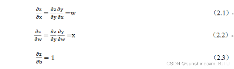
Computational graph is a kind of directed acyclic image , Graphically represent the relationship between operators and variables , Intuitive and efficient . Pictured 2-8 Shown , A circle represents a variable , Matrix representation operator . Like the expression ：z=wx+b, It can be written in two expressions ：$y=wx$, be $z=y+b$, among $x、w、b$ As a variable , Is a user created variable , Independent of other variables , So it is also called leaf node .
To calculate the gradient of each leaf node , You need to put the corresponding tensor parameter requires_grad Property is set to True, This automatically tracks its history .y、z Is the calculated variable , Nonleaf node ,z Root node .mul and add It's an operator （ Or operation or function ）. By these variables and operators , It constitutes a complete calculation process （ Or forward propagation process ）.

chart 2-8 Forward propagation calculation diagram
Our goal is to update the gradient of each leaf node , According to the chain rule of derivative of compound function , It is not difficult to calculate the gradient of each leaf node .

Pytorch call backward(), The gradient of each node will be calculated automatically , This is a back propagation process , This process can be illustrated by 2-9 Express . In the process of back propagation ,autograd Along the graph 2-9, From the current root node z Reverse traceability , Using the derivative chain rule , Calculate the gradient of all leaf nodes , Its gradient value will accumulate to grad Properties of the . Calculation of non leaf nodes （ or function） Recorded in the grad_fn Properties of the , Leaf node grad_fn The value is None.

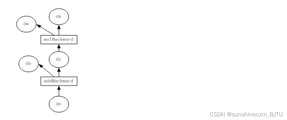
chart 2-9 Gradient back propagation calculation diagram
Let's implement this calculation diagram with code .

2.5.3 Scalar back propagation

hypothesis $x、w、b$ All scalars ,$z=wx+b$, For scalars $z$ call backward(), We don't need to be right backward() Pass in the parameter . The following are the main steps to realize automatic derivation ：
(1) Define leaf nodes and operator nodes

import torch
 
# Define the input tensor x
x=torch.Tensor([2])
# Initialize weight parameters W, Offset b、 And set up require_grad The attribute is True, For automatic derivation 
w=torch.randn(1,requires_grad=True)
b=torch.randn(1,requires_grad=True)
# Achieve forward propagation 
y=torch.mul(w,x)  # Equivalent to w*x
z=torch.add(y,b)  # Equivalent to y+b
# see x,w,b Of page child nodes requite_grad attribute 
print("x,w,b Of require_grad Properties are ：{},{},{}".format(x.requires_grad,w.requires_grad,b.requires_grad))

Running results
x,w,b Of require_grad Properties are ：False,True,True

（2） View leaf nodes 、 Other attributes of non leaf nodes

# View non leaf nodes requres_grad attribute ,
print("y,z Of requires_grad Properties are ：{},{}".format(y.requires_grad,z.requires_grad))
# Cause and w,b There is a dependency , so y,z Of requires_grad Properties are also ：True,True
# Check whether each node is a leaf node 
print("x,w,b,y,z Whether the node is a leaf node ：{},{},{},{},{}".format(x.is_leaf,w.is_leaf,b.is_leaf,y.is_leaf,z.is_leaf))
#x,w,b,y,z Whether the node is a leaf node ：True,True,True,False,False
# View the leaf node grad_fn attribute 
print("x,w,b Of grad_fn attribute ：{},{},{}".format(x.grad_fn,w.grad_fn,b.grad_fn))
# because x,w,b Created for the user , Is calculated by other tensors , so x,w,b Of grad_fn attribute ：None,None,None
# View non leaf nodes grad_fn attribute 
print("y,z Whether the node is a leaf node ：{},{}".format(y.grad_fn,z.grad_fn))
#y,z Whether the node is a leaf node ：,

（3） Automatic derivation , Realize gradient direction propagation , That is, the back propagation of the gradient .

# be based on z Tensor gradient back propagation , perform backward After that, the calculation chart will be automatically cleared ,
z.backward()
# If it needs to be used many times backward, Parameters need to be modified retain_graph by True, Now the gradient is cumulative 
#z.backward(retain_graph=True)
 
# View the gradient of leaf nodes ,x It's a leaf node, but it doesn't need derivation , So the gradient is None
print(" Parameters w,b And the gradients of these are :{},{},{}".format(w.grad,b.grad,x.grad))
# Parameters w,b And the gradients of these are :tensor([2.]),tensor([1.]),None
 
# Gradient of non leaf nodes , perform backward after , It will empty automatically 
print(" Nonleaf node y,z And the gradients of these are :{},{}".format(y.grad,z.grad))
# Nonleaf node y,z And the gradients of these are :None,None

2.5.4 Non scalar back propagation

2.5.3 In this section, we introduce when the target tensor is scalar , call backward() No parameters need to be passed in . The target tensor is generally scalar , Such as the loss value we often use Loss, It's usually a scalar . But there are also non scalar cases , What we will introduce later Deep Dream The target value of is a tensor with multiple elements . How to back propagate non scalars ？Pytorch There is a simple rule , Don't let the tensor (tensor) Take the derivative of the tensor , Only scalar derivatives of tensors are allowed , therefore , If the target tensor calls on a non scalar backward(), Need to pass in a gradient Parameters , This parameter is also a tensor , And you need to call backward() The shape of the tensor is the same . Why introduce a tensor gradient？

This parameter is passed in to convert tensor derivative to scalar derivative . It's a bit awkward , Let's take an example , Suppose the target value is $loss=(y_1,y_2,\dots ,y_m)$ The parameter passed in is $v=(v_1,v_2,\dots ,v_m)$ , Then you can put the right loss The derivation of , Convert to right $loss\ast v^T$ Derivative of scalar . That is, the original $\partial loss/\partial x$ Get the Jacobian matrix (Jacobian) Times the tensor $v^T$, Then we can get the gradient matrix we need .
backward The format of the function is ：

backward(gradient=None, retain_graph=None, create_graph=False)

It may be a little abstract , Let's illustrate with an example .
（1） Define leaf nodes and calculation nodes

import torch
 
# Define the leaf node tensor x, Shape is 1x2
x= torch.tensor([[2, 3]], dtype=torch.float, requires_grad=True)
# initialization Jacobian matrix 
J= torch.zeros(2 ,2)
# Initialize the target tensor , Shape is 1x2
y = torch.zeros(1, 2)
# Definition y And x Mapping between ：
#y1=x1**2+3*x2,y2=x2**2+2*x1
y[0, 0] = x[0, 0] ** 2 + 3 * x[0 ,1]
y[0, 1] = x[0, 1] ** 2 + 2 * x[0, 0]

（2） Calculate by hand y Yes x Gradient of
Let's calculate it manually first y Yes x Gradient of , In order to verify Pytorch Of backward Is the result of .
y Yes x The gradient of is a Jacobian matrix , The value of each item , We can calculate by the following method .

（3） call backward obtain y Yes x Gradient of

y.backward(torch.Tensor([[1, 1]]))
print(x.grad)
#  The result is tensor([[6., 9.]])

This result is inconsistent with our manual calculation , Obviously this result is wrong , What's wrong ？ The calculation process of this result is ：

thus , Wrong v Wrong value of , What you get in this way is not y Yes x Gradient of . Here we can divide the calculation into two steps . First let's v=(1,0) obtain y_1 Yes x Gradient of , Then make v=(0,1), obtain y_2 Yes x Gradient of . Here, it needs to be reused backward(), You need to make the parameters retain_graph=True, The specific code is as follows ：

# Generate y1 Yes x Gradient of 
y.backward(torch.Tensor([[1, 0]]),retain_graph=True)
J[0]=x.grad
# Gradients are cumulative , So we need to be right x The gradient is cleared 
x.grad = torch.zeros_like(x.grad)
# Generate y2 Yes x Gradient of 
y.backward(torch.Tensor([[0, 1]]))
J[1]=x.grad
# Show jacobian The value of matrix 
print(J)

Running results
tensor([[4., 3.],[2., 6.]])
This result is similar to the formula run manually （2.5） Consistent result .

2.6 Use Numpy Implement machine learning

We introduced Numpy、Tensor Basic content of , How to use Numpy、Tensor Operation array has a certain understanding . In order to deepen our understanding of Pytorch How to complete machine learning 、 Deep learning , The rest of this chapter will be divided into Numpy、Tensor、autograd、nn And optimal Implement the same machine learning task , Compare their similarities and differences and their respective advantages and disadvantages , So as to deepen the understanding of Pytorch The understanding of the .

First , We use the most primitive Numpy Implement a machine learning task about regression , no need Pytorch Package or class in . This method may have a little more code , But every step is transparent , It is helpful to understand the working principle of each step .
The main steps include ：
First , Is to give an array x, Then based on the expression ：$y=3x^2+2$, Add some noise data to another set of data y.
then , Build a machine learning model , Learn expressions $y=w{x}^2+b$ Two parameters of $w,b$. Using the array x,y The data is training data
Last , Using gradient descent method , Through many iterations , Learning to $w、b$ Value .
Here are the specific steps ：
（1） Import required libraries

# -*- coding: utf-8 -*-
import numpy as np
%matplotlib inline
 
from matplotlib import pyplot as plt

（2） Generate input data x And target data y
Set random number seed , Generate the same copy of data , In order to compare in many ways .

np.random.seed(100) 
x = np.linspace(-1, 1, 100).reshape(100,1) 
y = 3*np.power(x, 2) +2+ 0.2*np.random.rand(x.size).reshape(100,1) 

（3） see x,y Data distribution

#  drawing 
plt.scatter(x, y)
plt.show()

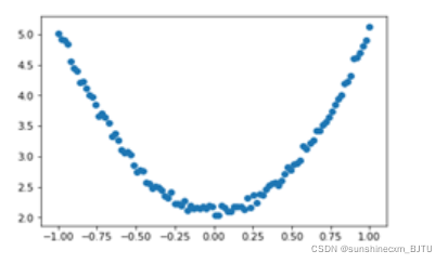
chart 2-10 Numpy Implemented source data
（4） Initialize weight parameters

#  Random initialization parameters 
w1 = np.random.rand(1,1)
b1 = np.random.rand(1,1) 

（5） Training models
Define the loss function , Suppose the batch size is 100：

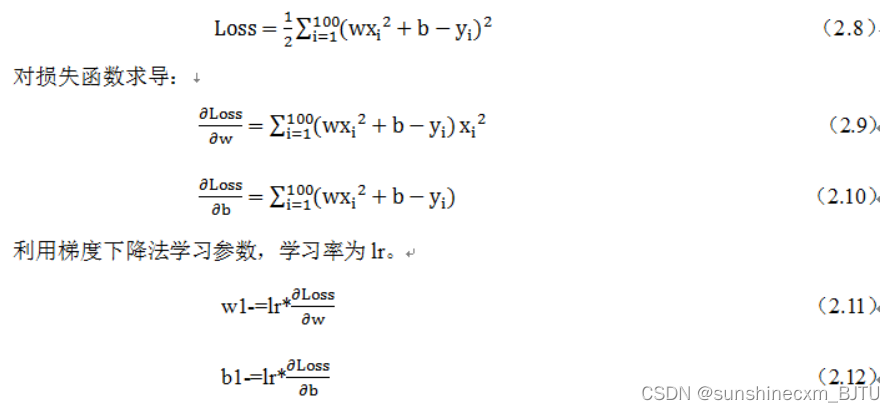
Implement the above expressions in code ：

lr =0.001 #  Learning rate 
 
for i in range(800):
    #  Forward propagation 
    y_pred = np.power(x,2)*w1 + b1
    #  Define the loss function 
    loss = 0.5 * (y_pred - y) ** 2
    loss = loss.sum()
    # Calculate the gradient 
    grad_w=np.sum((y_pred - y)*np.power(x,2))
    grad_b=np.sum((y_pred - y))
    # Using gradient descent , yes loss Minimum 
    w1 -= lr * grad_w
    b1 -= lr * grad_b

（6） Visualization results

plt.plot(x, y_pred,'r-',label='predict')
plt.scatter(x, y,color='blue',marker='o',label='true') # true data
plt.xlim(-1,1)
plt.ylim(2,6)  
plt.legend()
plt.show()
print(w1,b1)

Running results ：

chart 2-11 visualization Numpy Learning results

[[2.95859544]] [[2.10178594]]
As a result , The learning effect is still ideal .

2.7 Use Tensor And antograd Implement machine learning

2.6 This section can be said to complete a machine learning task by hand , The data used Numpy Express , Gradients and learning are learning models that you define and build . This method is suitable for relatively simple situations , If it's a little more complicated , The amount of code increases the geometric level . Is there a more convenient way ？ In this section, we will Use Pytorch A package of automatic derivation of antograd, Use this package and the corresponding Tensor, The gradient can be obtained by automatic back propagation , There is no need to calculate the gradient manually . The following is the specific implementation code .
（1） Import required libraries

import torch as t
%matplotlib inline
 
from matplotlib import pyplot as plt

（2） Generate training data , And visualize the data distribution

t.manual_seed(100) 
dtype = t.float
# Generate x Coordinate data ,x by tenor, Need to put x Convert the shape of to 100x1
x = t.unsqueeze(torch.linspace(-1, 1, 100), dim=1) 
# Generate y Coordinate data ,y by tenor, Shape is 100x1, Plus some noise 
y = 3*x.pow(2) +2+ 0.2*torch.rand(x.size())                 
 
#  drawing , hold tensor Data to numpy data 
plt.scatter(x.numpy(), y.numpy())
plt.show()

chart 2-12 Visual input data
（3） Initialize weight parameters

#  Random initialization parameters , Parameters w,b For those who need to learn , Therefore, we need requires_grad=True
w = t.randn(1,1, dtype=dtype,requires_grad=True)
b = t.zeros(1,1, dtype=dtype, requires_grad=True) 

（4） Training models

lr =0.001 #  Learning rate 
 
for ii in range(800):
    #  Forward propagation , And define the loss function loss
    y_pred = x.pow(2).mm(w) + b
    loss = 0.5 * (y_pred - y) ** 2
    loss = loss.sum()
    
    #  Automatically calculate gradients , The gradient is stored in grad Properties of the 
    loss.backward()
    
    #  Manually update parameters , Need to use torch.no_grad(), Make the calculation of automatic derivation cut off in the context 
    with t.no_grad():
        w -= lr * w.grad
        b -= lr * b.grad
    
    #  Gradient clear 
        w.grad.zero_()
        b.grad.zero_()

（5） Visualizing training results

plt.plot(x.numpy(), y_pred.detach().numpy(),'r-',label='predict')#predict
plt.scatter(x.numpy(), y.numpy(),color='blue',marker='o',label='true') # true data
plt.xlim(-1,1)
plt.ylim(2,6)  
plt.legend()
plt.show()
        
print(w, b)

Running results ：

chart 2-13 Use antograd Result
tensor([[2.9645]], requires_grad=True) tensor([[2.1146]], requires_grad=True)
This result is consistent with the use of Numpy Machine learning is similar .