Summary of Wu Enda's course of machine learning (4)

12. Chapter 12 Support vector machine （Support Vector Machines,SVM）

12.1 Optimization objectives （optimization objective）

1. Another view of logistic regression

   $h_{\theta }(x)=\frac{1}{1+e^{-{\theta }^{T}x}}$

   • Such as $y=1$, We want to $h_{\theta }(x)\approx 1$, namely $e^{-{\theta }^{T}x}\gg 0$
   • Such as $y=0$, We want to $h_{\theta }(x)\approx 0$, namely $e^{-{\theta }^{T}x}\ll 0$

   $\cos t(h_{\theta }(x),y)=-(\mathrm{y}\log (h_{\theta }(x))+(1-\mathrm{y})\log (1-h_{\theta }(x)))=-y\log (\frac{1}{1+e^{-{\theta }^{T}x}})-(1-y)\log (1-\frac{1}{1+e^{-{\theta }^{T}x}})$

   

   Use $\cos t_1(z),\cos t_0(z)$ To replace separately $-\log (\frac{1}{1+e^{-{\theta }^{T}x}}),-\log (1-\frac{1}{1+e^{-{\theta }^{T}x}})$

2. SVM

$\underset{\theta }{\min }C\sum _{i=1}^m[y^{(i)}\cos t_1({\theta }^T{x}^{(i)})+(1-y^{(i)})\cos t_0({\theta }^T{x}^{(i)})]+\frac{1}{2}\sum _{j=1}^n{{\theta }_j}^2$,$C$ Constant

SVM Assume no output probability , Make direct predictions ：

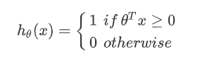
12.2 Large interval visual understanding （Large Margin Intuition）

$\underset{\theta }{\min }C\sum _{i=1}^m[y^{(i)}\cos t_1({\theta }^T{x}^{(i)})+(1-y^{(i)})\cos t_0({\theta }^T{x}^{(i)})]+\frac{1}{2}\sum _{j=1}^n{{\theta }_j}^2$

• Such as $y=1$, We want to ${\theta }^{T}x\ge 1$, Not just $\ge 0$
• Such as $y=0$, We want to ${\theta }^{T}x\ge -1$, Not just $\le 0$

SVM Decision boundaries （SVM Decision Boundary）： Linearly separable case , Interval of support vector machine ,$\underset{\theta }{\min }C0+\frac{1}{2}\sum _{j=1}^n{{\theta }_j}^2$

• $C$ Very big time , Want to classify the samples in each training set correctly , Sensitive to noise
• $C$ Not very big , Partial sample classification error is allowed , Insensitive to noise , Even in the case of linear inseparability ,SVM Can also do well .
• $C$ amount to $\frac{1}{\lambda }$

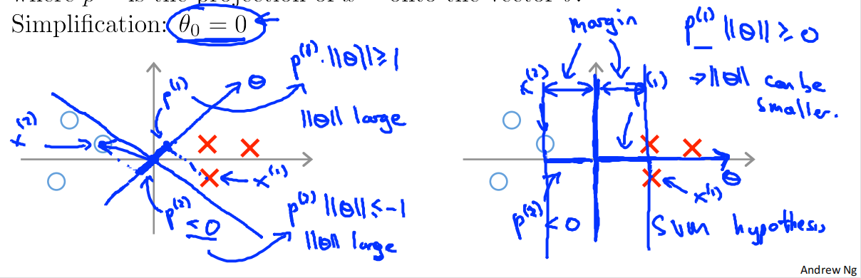
12.3 Mathematical principle of large interval classifier

Appointment ：

$\parallel u\parallel =lengthofvectoru=\sqrt{u_1^2+u_2^2}\in R$

$P$ be equal to $v$ stay $u$ Mapping on ,$u^{T}v=P\bullet \parallel u\parallel =u_1{v}_1+u_2{v}_2\in R$.

Decision boundaries ：$\underset{\theta }{\min }\frac{1}{2}\sum _{j=1}^n{{\theta }_j}^2$,$C$ Very big time .

Simplified analysis ：${\theta }_0=0,n=2$

$\frac{1}{2}\sum _{j=1}^n{{\theta }_j}^2=\frac{1}{2}({\theta }_1^2+{\theta }_2^2)=\frac{1}{2}(\sqrt{{\theta }_1^2+{\theta }_2^2}{)}^2=\frac{1}{2}\parallel \theta {\parallel }^2$

${\theta }^T{x}^{(i)}=P^{(i)}+\parallel \theta \parallel ={\theta }_1{x}_1^{(i)}+{\theta }_2{x}_2^{(i)}$

12.4 Kernel function 1（Kernels）

Nonlinear decision boundary ：

When ${\theta }_0+{\theta }_1{x}_1+{\theta }_2{x}_2+{\theta }_3{x}_1{x}_2+{\theta }_4{x_1}^2+{\theta }_5{x_2}^2+...\ge 0$, forecast $y=1$.

Define new features ：$f_1=x_1,f_2=x_2,f_3=x_1{x}_2,...$, Is there a better way ？

Given $x$, The calculation of new features depends on the connection with landmarks （$l^{(1)},l^{(2)},l^{(3)}$） The proximity of .

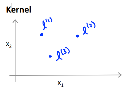
$f_1=similarity(x,l^{(1)})=\exp (-\frac{\parallel x-l^{(1)}{\parallel }^2}{2{\sigma }^2})$, To measure $x,l^{(1)}$ The similarity .

The kernel function is marked as ：$\kappa (x,l^{(i)})$

12.5 Kernel function 2

How to get $l^{(1)},l^{(2)},l^{(3)},...$？

With kernel function SVM：

• Training set ： { ( x ( 1 ) , y ( 1 ) ) , ( x ( 2 ) , y ( 2 ) ) , . . . , ( x ( m ) , y ( m ) ) } \{ ({x^{(1)}},{y^{(1)}}),({x^{(2)}},{y^{(2)}}),...,({x^{(m)}},{y^{(m)}})\} { (x(1),y(1)),(x(2),y(2)),...,(x(m),y(m))}
• choice $l^{(1)}=x^{(1)},l^{(2)}=x^{(2)},...,l^{(m)}=x^{(m)}$
• Calculation $f$：$f_1=similarity(x,l^{(1)})$,…,$f_m=similarity(x,l^{(m)})$,$f$ As a feature of training
• $\underset{\theta }{\min }C\sum _{i=1}^m[y^{(i)}\cos t_1({\theta }^T{f}^{(i)})+(1-y^{(i)})\cos t_0({\theta }^T{f}^{(i)})]+\frac{1}{2}\sum _{j=1}^n{{\theta }_j}^2$

Why not apply the kernel technique to logistic regression , Because when combined with logistic regression, it becomes very slow , Some optimizations are for kernel functions and SVM Of .

SVM Parameters ：

• $C(=\frac{1}{\lambda })$：
  • Big $C$： Low deviation , High variance —— Over fitting
  • Small $C$： High deviation , Low variance —— Under fitting
• ${\sigma }^2$：
  • Big ${\sigma }^2$： features $f$ Very smooth . High deviation , Low variance —— Under fitting
  • Small ${\sigma }^2$： features $f$ Very uneven . High deviation , Low deviation , High variance —— Over fitting

12.6 Use SVM

Use SVM The software package solves the parameter $\theta$ Calculation problem .

Pay attention to two points ：

• Parameters $C$ The choice of
• The choice of kernel function

1. Kernel free function （ Linear kernel function ）, Get a linear classifier . When $n$ It's big ,$m$ Very feasible . however , In a very high dimensional feature space , Try fitting very complex functions , If the training set is small , Maybe over fitting .

2. Gaussian kernel （Gaussian kernel）：

   $f_i=\exp (-\frac{\parallel x-l^{(1)}{\parallel }^2}{2{\sigma }^2})$

   Need to choose ${\sigma }^2$

   When $n$ Very small ,$m$ When it is very large, it can fit the nonlinear .

Kernel function note ： If the value range of the original feature is very different , Probably $f$ It is largely determined by only some characteristics .

Other kernel functions ：String kernel,chiIsquare’kernel, histogram intersec2on’kernel,…

Be careful ： Not all similarity functions $similarity(x,l)$ Are valid cores .( Need to meet the requirements named " Mercer's Theorem " Technical conditions of , In order to ensure that SVM Package optimization works correctly , And don't disagree ）.

Many classification ：

many SVM The learning package has built-in multi classification methods , Use one to many for multi classification .

Logical regression VS SVM：

$n$ Represents the number of features ,$m$ Indicates the number of training samples

1. If $n$ relative $m$ It's big （ Such as ：$n=10000,m=10\sim 1000$）, Using logistic regression or linear kernel function SVM
2. If $n$ smaller $m$ secondary （ Such as ：$n=1\sim 1000,m=10\sim 10000$）, Using Gaussian kernel function SVM
3. If $n$ smaller $m$ It's big （ Such as ：$n=1\sim 1000,m=50000+$）, Using logistic regression or linear kernel function SVM

Neural networks may perform well in most cases , But training may be slower .

13. clustering （Clustering）

13.1 Unsupervised learning （Unsupervised Learning Introduction）

Training set ： { x ( 1 ) , x ( 2 ) , . . . , x ( m ) } \{ {x^{(1)}},{x^{(2)}},...,{x^{(m)}}\} { x(1),x(2),...,x(m)}

Application of clustering algorithm ： Market segmentation ; Social network analysis ; Server organization ; Astronomical data analysis

13.2 K Mean clustering algorithm （k-means algorithm）

K Mean clustering algorithm ：

• Input ：K（ Number of clusters ）; Training set ： { x ( 1 ) , x ( 2 ) , . . . , x ( m ) } \{ {x^{(1)}},{x^{(2)}},...,{x^{(m)}}\} { x(1),x(2),...,x(m)},$x^{(i)}\in R^n$ Default $x_0^{}=1$
• Random initialization K Class center $u_1,u_2,...,u_k\in R^n$
• Cluster allocation （cluster assignment step）： Assign each point to the nearest class center point .（ New clustering ）
• Update cluster center （move centroid）： Calculate the mean value of each type of data point as the new class center .（ New center ）
• Repeat the above steps until convergence , That is, the clustering result remains unchanged

13.3 Optimization objectives （Optimization objective）

$c^{(i)}$ Express $x^{(i)}$ Which category is currently assigned to ;$u_k$ Represents the class center k;$u_{c^{(i)}}$ Express $x^{(i)}$ Which class center is currently assigned to .

Optimization objectives ：$J(c^{(1)},...,c^{(m)},...,u_1,...,u_K)=\frac{1}{m}\sum _{i=1}^m\parallel x^{(i)}-u_{c^{(i)}}{\parallel }^2$

$\underset{c^{(1)},...,c^{(m)},...,u_1,...,u_K}{\min }J(c^{(1)},...,c^{(m)},...,u_1,...,u_K)$

Can prove that ：

• First step ： Cluster allocation （ New clustering ） Is optimizing $c^{(1)},...,c^{(m)}$, And keep $u_1,...,u_K$ unchanged
• The second step ： Update cluster center （ New center ） Is optimizing $u_1,...,u_K$, And keep $c^{(1)},...,c^{(m)}$ unchanged
• k-means In fact, it is minimized in two steps $J(c^{(1)},...,c^{(m)},...,u_1,...,u_K)=\frac{1}{m}\sum _{i=1}^m\parallel x^{(i)}-u_{c^{(i)}}{\parallel }^2$, Then iterate repeatedly until convergence

13.4 Random initialization （Random initialization）

The following conditions are met ：

• Should have $K<m$
• Random selection $K$ Training samples
• Set up $u_1,...,u_K$ It's equal to this $K$ Training samples

Due to different initialization ,K The mean clustering algorithm may fall into the local optimum . To solve the local optimum , especially $K=2\sim 10$ when , Adopting the following scheme has greatly improved ： Run repeatedly 50~1000 Time k-means Take the best .

13.5 Select the number of clusters （Choosing the number of clusters）

1. “ Elbow ” Law （Elbow method）：

Can solve some problems , But you can't deal with all the problems .

2. Sometimes , You are running k-means De clustering , For the next step . This can be based on the performance of the next work , As an option $K$ Principle of .

14. Chapter 14 Dimension reduction （Dimensionality Reduction）

14.1 The goal is 1： data compression

Purpose ： To reduce the space ; Algorithm acceleration

Reduce the amount of data , Such as ： Two dimensions to one dimension , 3D to 2D

The dimension of a matrix is generally the number of values in a vector , Be careful ： The vector is vertical by default

14.2 The goal is 2： visualization

High dimensional data is often mapped to 3D or 2D for visualization .

14.3 Principal component analysis problem planning （Principal Component Analysis,PCA）

Problem description ： Reduce the quantity n Dimension to k dimension , Search for k Base vectors $u^{(1)},u^{(2)},...,u^{(k)}$ Represents all data , And mapping errors are minimal .

PCA Not linear regression .

14.4 Principal component analysis algorithm （Principal Component Analysis,PCA）

Training set ： { x ( 1 ) , x ( 2 ) , . . . , x ( m ) } \{ {x^{(1)}},{x^{(2)}},...,{x^{(m)}}\} { x(1),x(2),...,x(m)}

1. Data preprocessing ： Including feature scaling or mean averaging .

   Calculation $u_j=\frac{1}{m}\sum _{i=1}^m{x}_j^{(i)}$, Then substitute $\frac{x_j-u_j}{s_j}$ On behalf of $x_j^{(i)}$.

   If the range of different features is different , Feature scaling is very necessary .k Dimensional space is primitive n Low dimensional subspaces of dimensional spaces （dimensional sub-space）

2. Calculate the covariance matrix （convariance matrix）

   $\Sigma =\frac{1}{m}\sum _{i=1}^m(x^{(i)}){(x^{(i)})}^T$, among $\Sigma$ yes $sigma$ matrix .

3. Calculate singular value decomposition （eigenvectors of sigma）

   $[u,s,v]=svd(sigma)$, among $u$ That's what we need

   $u=\left[\underset{k}{\underbrace{u^{(1)},u^{(2)}}},...,u^{(m)}\right]\in R^{n\times n}$, take $u$ Before k Just a vector .

4. $x\in R^n\Rightarrow z\in R^k$

   KaTeX parse error: Undefined control sequence: \matrix at position 86: …(i)}} = \left[ \̲m̲a̲t̲r̲i̲x̲{ {u^{(1)}} \…

14.5 Main component fraction selection

Square mean of mapping error ：$\frac{1}{m}\sum _{i=1}^m\parallel x^{(i)}-x_{approix}^{(i)}{\parallel }^2$; Total data change ：$\frac{1}{m}\sum _{i=1}^m\parallel x^{(i)}{\parallel }^2$

Try to choose k Minimize the following values , That is to maximize the retention of all differences ：

$\frac{\frac{1}{m}\sum _{i=1}^m\parallel x^{(i)}-x_{approix}^{(i)}{\parallel }^2}{\frac{1}{m}\sum _{i=1}^m\parallel x^{(i)}{\parallel }^2}\le 0.01$, Equivalent to 99% The variance of is retained

choice k Methods ：

Try different k The value of ,$k=1,2,...$, Calculation $z^{(1)},z^{(2)},...,z^{(m)},x_{approix}^{(1)},x_{approix}^{(2)},...,x_{approix}^{(m)}$, Check to see if $\frac{\frac{1}{m}\sum _{i=1}^m\parallel x^{(i)}-x_{approix}^{(i)}{\parallel }^2}{\frac{1}{m}\sum _{i=1}^m\parallel x^{(i)}{\parallel }^2}\le 0.01$. But this calculation is too expensive , You can use $[u,s,v]=svd(sigma)$ Medium $s$ Calculation .

$\frac{\frac{1}{m}\sum _{i=1}^m\parallel x^{(i)}-x_{approix}^{(i)}{\parallel }^2}{\frac{1}{m}\sum _{i=1}^m\parallel x^{(i)}{\parallel }^2}\le 0.01\Rightarrow 1-\frac{\sum _{i=1}^k{s}_{ii}}{\sum _{i=1}^n{s}_{ii}}\le 0.01$,k Traverse from small to large and select the smallest one that satisfies the condition k.

14.6 Compression reproduction

$Z=U^{T}X\Rightarrow X_{approix}=UZ\approx X$

14.6 application PCA The advice of

Supervised learning accelerates ：

Training set ： { ( x ( 1 ) , y ( 1 ) ) , ( x ( 2 ) , y ( 2 ) ) , . . . , ( x ( m ) , y ( m ) ) } \{ ({x^{(1)}},{y^{(1)}}),({x^{(2)}},{y^{(2)}}),...,({x^{(m)}},{y^{(m)}})\} { (x(1),y(1)),(x(2),y(2)),...,(x(m),y(m))}

Perform on the input PCA, { ( x ( 1 ) , y ( 1 ) ) , ( x ( 2 ) , y ( 2 ) ) , . . . , ( x ( m ) , y ( m ) ) } ⇒ { ( z ( 1 ) , y ( 1 ) ) , ( z ( 2 ) , y ( 2 ) ) , . . . , ( z ( m ) , y ( m ) ) } \{ ({x^{(1)}},{y^{(1)}}),({x^{(2)}},{y^{(2)}}),...,({x^{(m)}},{y^{(m)}})\} \Rightarrow \{ ({z^{(1)}},{y^{(1)}}),({z^{(2)}},{y^{(2)}}),...,({z^{(m)}},{y^{(m)}})\} { (x(1),y(1)),(x(2),y(2)),...,(x(m),y(m))}⇒{ (z(1),y(1)),(z(2),y(2)),...,(z(m),y(m))}.

Be careful ： On the training set PCA Mapping calculation , However, the mapping can be applied to validation sets and test sets .

application PCA：

• Compress ：
  • Reduce memory footprint
  • Learning algorithm acceleration
• visualization

1. Do not use PCA To solve the fitting problem .
2. When is not suitable for use PCA？ First, experiment with the original input , If the desired effect is not achieved , Consider adopting PCA.PCA After all, it is dimensionality reduction , There will still be a loss of information ！ And it adds extra work .