当前位置:网站首页>深度学习100例 —— 循环神经网络(RNN)实现股票预测
深度学习100例 —— 循环神经网络(RNN)实现股票预测
2022-08-09 22:03:00 【Ding Jiaxiong】
活动地址:CSDN21天学习挑战赛
深度学习100例——循环神经网络(RNN)实现股票预测
- 本文为365天深度学习训练营 中的学习记录博客
- 参考文章地址: 深度学习100例-循环神经网络(RNN)实现股票预测 | 第9天
文章目录
我的环境

1 RNN
1.1 RNN简介
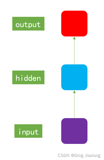
传统神经网络结构:
- 输入层
- 隐藏层
- 输出层
RNN和传统神经网络ANN的最大的区别在于每次会将前一次的输出结果,带到下一次迭代的隐藏层中,一起进行训练。
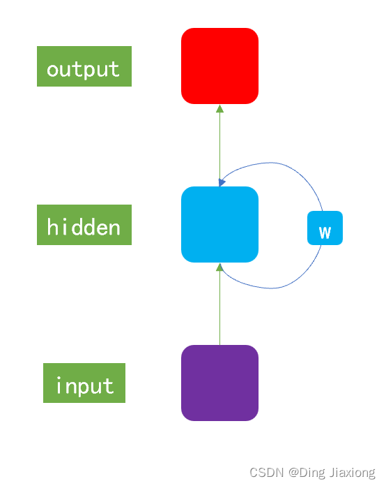
一般以序列数据作为输入,通过网络的内部结构设计有效捕捉序列之间的关系特征,一般也以序列形式进行输出。
1.2 RNN模型作用
- 很好地利用序列之间的关系 → 针对自然界具有连续性的输入序列,能进行很好地处理。
- 适用场景
- 文本分类
- 情感分析
- 意图识别
- 机器翻译
2 准备工作
2.1 设置GPU
import tensorflow as tf

gpus = tf.config.list_physical_devices("GPU")

if gpus:
    tf.config.experimental.set_memory_growth(gpus[0], True)  #设置GPU显存用量按需使用
    tf.config.set_visible_devices([gpus[0]],"GPU")

2.2 加载数据
import os,math
from tensorflow.keras.layers import Dropout, Dense, SimpleRNN
from sklearn.preprocessing import MinMaxScaler
from sklearn import metrics
import numpy             as np
import pandas            as pd
import tensorflow        as tf
import matplotlib.pyplot as plt
# 支持中文
plt.rcParams['font.sans-serif'] = ['SimHei']  # 用来正常显示中文标签
plt.rcParams['axes.unicode_minus'] = False  # 用来正常显示负号

读入股票文件
data = pd.read_csv('SH600519.csv')  # 读取股票文件
data

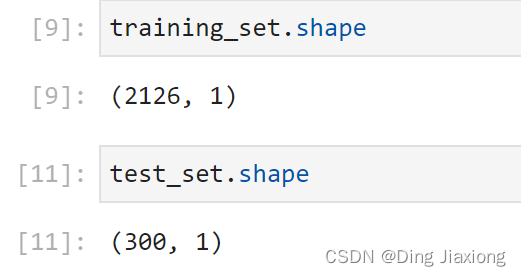
划分数据集合
前(2426-300=2126)天的开盘价作为训练集,表格从0开始计数,2:3 是提取[2:3)列,前闭后开,故提取出C列开盘价后300天的开盘价作为测试集
training_set = data.iloc[0:2426 - 300, 2:3].values
test_set = data.iloc[2426 - 300:, 2:3].values
3 数据预处理
3.1 归一化
sc = MinMaxScaler(feature_range=(0, 1))
training_set = sc.fit_transform(training_set)
test_set = sc.transform(test_set)
3.2 设置测试集、训练集
x_train = []
y_train = []

x_test = []
y_test = []

""" 使用前60天的开盘价作为输入特征x_train 第61天的开盘价作为输入标签y_train for循环共构建2426-300-60=2066组训练数据。 共构建300-60=260组测试数据 """
for i in range(60, len(training_set)):
    x_train.append(training_set[i - 60:i, 0])
    y_train.append(training_set[i, 0])

for i in range(60, len(test_set)):
    x_test.append(test_set[i - 60:i, 0])
    y_test.append(test_set[i, 0])

# 对训练集进行打乱
np.random.seed(7)
np.random.shuffle(x_train)
np.random.seed(7)
np.random.shuffle(y_train)
tf.random.set_seed(7)
""" 将训练数据调整为数组(array) 调整后的形状: x_train:(2066, 60, 1) y_train:(2066,) x_test :(240, 60, 1) y_test :(240,) """
x_train, y_train = np.array(x_train), np.array(y_train) # x_train形状为:(2066, 60, 1)
x_test,  y_test  = np.array(x_test),  np.array(y_test)

""" 输入要求:[送入样本数, 循环核时间展开步数, 每个时间步输入特征个数] """
x_train = np.reshape(x_train, (x_train.shape[0], 60, 1))
x_test  = np.reshape(x_test,  (x_test.shape[0], 60, 1))

4 构建模型
model = tf.keras.Sequential([
    SimpleRNN(100, return_sequences=True), #布尔值。是返回输出序列中的最后一个输出,还是全部序列。
    Dropout(0.1),                         #防止过拟合
    SimpleRNN(100),
    Dropout(0.1),
    Dense(1)
])
5 激活模型
# 该应用只观测loss数值,不观测准确率,所以删去metrics选项,一会在每个epoch迭代显示时只显示loss值
model.compile(optimizer=tf.keras.optimizers.Adam(0.001),loss='mean_squared_error')  # 损失函数用均方误差
6 训练模型
history = model.fit(x_train, y_train,
                    batch_size=64,
                    epochs=20,
                    validation_data=(x_test, y_test),
                    validation_freq=1)                  #测试的epoch间隔数

model.summary()

7 结果可视化
7.1 绘制loss
plt.plot(history.history['loss']    , label='Training Loss')
plt.plot(history.history['val_loss'], label='Validation Loss')
plt.title('Training and Validation Loss by DingJiaxiong')
plt.legend()
plt.show()

7.2 预测
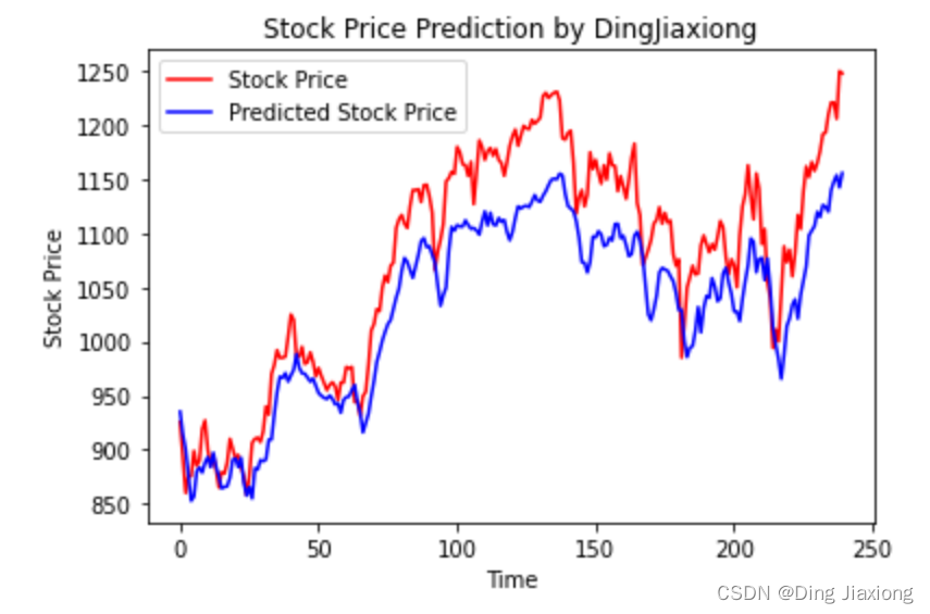
predicted_stock_price = model.predict(x_test)                       # 测试集输入模型进行预测
predicted_stock_price = sc.inverse_transform(predicted_stock_price) # 对预测数据还原---从(0,1)反归一化到原始范围
real_stock_price = sc.inverse_transform(test_set[60:])              # 对真实数据还原---从(0,1)反归一化到原始范围

# 画出真实数据和预测数据的对比曲线
plt.plot(real_stock_price, color='red', label='Stock Price')
plt.plot(predicted_stock_price, color='blue', label='Predicted Stock Price')
plt.title('Stock Price Prediction by DingJiaxiong')
plt.xlabel('Time')
plt.ylabel('Stock Price')
plt.legend()
plt.show()
7.3 评估
""" MSE :均方误差 -----> 预测值减真实值求平方后求均值 RMSE :均方根误差 -----> 对均方误差开方 MAE :平均绝对误差-----> 预测值减真实值求绝对值后求均值 R2 :决定系数,可以简单理解为反映模型拟合优度的重要的统计量 """
MSE   = metrics.mean_squared_error(predicted_stock_price, real_stock_price)
RMSE  = metrics.mean_squared_error(predicted_stock_price, real_stock_price)**0.5
MAE   = metrics.mean_absolute_error(predicted_stock_price, real_stock_price)
R2    = metrics.r2_score(predicted_stock_price, real_stock_price)

print('均方误差: %.5f' % MSE)
print('均方根误差: %.5f' % RMSE)
print('平均绝对误差: %.5f' % MAE)
print('R2: %.5f' % R2)

边栏推荐
猜你喜欢
Quotefancy ,提供鼓舞人心语录的壁纸网站 - 倾城之链

Presto Event Listener开发
Js fifteen interview questions (with answers)
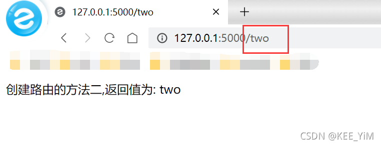
Flask's routing (app.route) detailed
![This article lets you quickly understand implicit type conversion [integral promotion]!](/img/16/4edc7ef23384b22d50ebd894b8911a.png)
This article lets you quickly understand implicit type conversion [integral promotion]!

金山云地震,震源在字节?
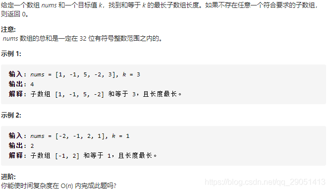
leetcode:325. 和等于k的最长子数组长度
JS解混淆-AST还原案例
leetcode:319. 灯泡开关

Arcgis工具箱无法使用,显示“XML包含错误“的解决方法

随机推荐
xctf攻防世界 Web高手进阶区 ics-05
Rust dereference
Under the NVM node installation;The node environment variable configuration
How do task flow executors work?
One Pass 2074: [21CSPJ Popularization Group] Candy
【Apifox】为什么如此受青睐,此篇文章和大家分享
大型分布式存储方案MinIO介绍,看完你就懂了!
nvm下node安装;node环境变量配置
openGauss数据库基本操作(超详细)
Linux 配置MySQL
R语言使用mean函数计算样本(观测)数据中指定变量的相对频数:计算时间序列数据中大于前一个观测值的观测值所占的比例总体的比例
一文让你快速了解隐式类型转换【整型提升】!
Five Star Holdings Wang Jianguo: Deepen the track with "plant spirit" and promote growth with "animal spirit"
注意力引导网络用于视网膜图像分割
three.js镂空圆球拖拽变形js特效
JS解混淆-AST还原案例
OSG笔记:使用setFontResolution设置字体分辨率
xctf攻防世界 Web高手进阶区 shrine
阿里云架构师金云龙:基于云XR平台的视觉计算应用部署
工作经验-组件封装(拖拽排序组件)