当前位置:网站首页>Machine learning theory (6): from logistic regression (logarithmic probability) method to SVM; Why is SVM the maximum interval classifier
Machine learning theory (6): from logistic regression (logarithmic probability) method to SVM; Why is SVM the maximum interval classifier
2022-04-22 03:38:00 【Warm baby can fly】
List of articles
Review the logarithmic probability
- In my last article :https://blog.csdn.net/qq_42902997/article/details/124255802?spm=1001.2014.3001.5501 The principle of logistic regression and optimization objectives are described in :
- Performed at each gradient descent step in , We all need to calculate each sample , For samples x i x_i xi, Its label is y i y_i yi, The vector of the parameter he needs to calculate can be expressed as θ T \theta^T θT( That includes b b b)
- We can argue that θ T ⋅ x i \theta^T\cdot x_i θT⋅xi after sigmoid The result of function processing is y i ^ \hat{y_i} yi^ namely , y i ^ = σ ( θ T ⋅ x i ) \hat{y_i}=\sigma(\theta^T\cdot x_i) yi^=σ(θT⋅xi)
- In this case , Our loss for each sample can be expressed as : L ( y i , y i ^ ) L(y_i, \hat{y_i}) L(yi,yi^) Again because y i y_i yi There are two different situations for the value of , We use a formula to express the optimization objectives in these two different cases L ( y i , y i ^ ) = − y i ^ y i ( 1 − y i ^ ) 1 − y i L(y_i, \hat{y_i})=-\hat{y_i}^{y_i}(1-\hat{y_i})^{1-y_i} L(yi,yi^)=−yi^yi(1−yi^)1−yi, after l o g log log After transformation, the final loss function for a sample is obtained : L ( y i , y i ^ ) = − y i l o g ( y i ^ ) + ( 1 − y i ) l o g ( 1 − y i ^ ) ( 1 ) L(y_i, \hat{y_i})=-{y_i}log(\hat{y_i})+({1-y_i})log(1-\hat{y_i})~~~~~~~~~~(1) L(yi,yi^)=−yilog(yi^)+(1−yi)log(1−yi^) (1)
- thus , Extend to the entire dataset m m m The total cost function of a sample can be written as : − 1 m Σ i = 1 m y i l o g ( y i ^ ) + ( 1 − y i ) l o g ( 1 − y i ^ ) + λ 2 m Σ j = 1 n θ j 2 ( 2 ) -\frac{1}{m}\Sigma_{i=1}^m{y_i}log(\hat{y_i})+({1-y_i})log(1-\hat{y_i})+\frac{\lambda}{2m}\Sigma_{j=1}^n\theta_j^2~~~~~~~~~~(2) −m1Σi=1myilog(yi^)+(1−yi)log(1−yi^)+2mλΣj=1nθj2 (2)
The second part of the formula is the regularization part
- The core of logarithmic probability is the introduction of sigmoid Nonlinear functions , Thus, the task of linear regression can evolve into a classification task ,sigmoid Function as follows :

- The symbols here θ T x \theta^Tx θTx It means the same as the above , there z = θ T x z=\theta^Tx z=θTx In fact, it is equivalent to y i ^ \hat{y_i} yi^
- When this x x x The corresponding real label is y = 1 y=1 y=1 When ( Positive samples ), We hope h θ ( x ) h_\theta(x) hθ(x) The value of is best approximated infinitely 1 1 1, In other words , We want to be sigmoid Before mapping θ T x \theta^Tx θTx The bigger the better , namely θ T x > > 0 \theta^Tx>>0 θTx>>0
- And when y = 0 y=0 y=0 When ( Negative sample ), And we hope h θ ( x ) h_\theta(x) hθ(x) The value of is best approximated infinitely 0 0 0, namely θ T x < < 0 \theta^Tx<<0 θTx<<0
Another perspective of logistic regression cost function
- Look at the formula (1) The cost function given :
L ( y i , y i ^ ) = − y i l o g ( y i ^ ) + ( 1 − y i ) l o g ( 1 − y i ^ ) L(y_i, \hat{y_i})=-{y_i}log(\hat{y_i})+({1-y_i})log(1-\hat{y_i}) L(yi,yi^)=−yilog(yi^)+(1−yi)log(1−yi^)
- If you write the formula more completely , Into the h θ ( x ) h_\theta(x) hθ(x) The definition of , And remove the subscript i i i ( Because we don't study all the samples in the whole data set for the time being , We only study the case of one sample , Not for the time being i i i To distinguish samples ) We can get the following formula :
L ( y , y ^ ) = − y l o g ( 1 1 + e − θ T x ) + ( 1 − y ) l o g ( 1 − 1 1 + e − θ T x ) = y ( − l o g ( 1 1 + e − θ T x ) ) + ( 1 − y ) l o g ( 1 − 1 1 + e − θ T x ) ( 3 ) L(y, \hat{y})=-{y}log(\frac{1}{1+e^{-\theta^Tx}})+({1-y})log(1-\frac{1}{1+e^{-\theta^Tx}}) \\= {y}(-log(\frac{1}{1+e^{-\theta^Tx}}))+({1-y})log(1-\frac{1}{1+e^{-\theta^Tx}}) ~~~~~~~~~~(3) L(y,y^)=−ylog(1+e−θTx1)+(1−y)log(1−1+e−θTx1)=y(−log(1+e−θTx1))+(1−y)log(1−1+e−θTx1) (3)
In this formula (3) Let's take a look at it alone y = 1 y=1 y=1 and y = 0 y=0 y=0 The case when , Look at the goals they want to optimize :
- When y = 1 y=1 y=1 When ( θ T x > > 0 ) \theta^Tx>>0) θTx>>0) By analyzing the formula (3) Only the first half is left − l o g ( 1 1 + e − θ T x ) -log(\frac{1}{1+e^{-\theta^Tx}}) −log(1+e−θTx1), This will be θ T x = z \theta^Tx=z θTx=z We can get a follow z z z Curve of value change :

- When z z z When the value of gradually increases , The value of this function tends to 0 0 0 Of
- That explains , Why to be y = 1 y=1 y=1 Usually when θ T x \theta^Tx θTx Set it very big . This is because in the y = 1 y=1 y=1 The whole loss function L ( y , y ^ ) L(y,\hat{y}) L(y,y^) There's only... Left − l o g ( 1 1 + e z ) -log(\frac{1}{1+e^z}) −log(1+ez1) At this time, set a big θ T x \theta^Tx θTx It's going to lead to the whole thing L ( y , y ^ ) L(y,\hat{y}) L(y,y^) Very small , It will reduce as much as possible loss Purpose .
- Empathy , about y = 0 y=0 y=0 The situation of , You can also see a curve when you come L ( y , y ^ ) L(y,\hat{y}) L(y,y^):

- You can also draw an intuitive conclusion from this diagram , When y = 0 y=0 y=0 When , take θ T x \theta^Tx θTx The setting is small , Because this time will also lead to L ( y , y ^ ) L(y,\hat{y}) L(y,y^) Very small
SVM Improvement
-
SVM It can be seen as improving the loss function on the basis of logarithmic probability regression ,logistic regression The loss function can be divided into two parts , It has also been discussed above , Look at here SVM The design of the , He put the two parts in 1 1 1 and − 1 -1 −1 Pull the value between to 0 0 0 了 , It's hard y = 1 y=1 y=1 and y = 0 y=0 y=0 A gap has been dug between the situation of .

-
In this case, how to express in mathematical form SVM What about the loss function of ?
-
Let's put the original formula (3) The loss in is divided into two parts , The front part is written as c o s t 1 ( z ) generation On behalf of − l o g ( 1 1 + e − z ) ( 4 ) cost_1(z) ~~ Instead of ~~-log(\frac{1}{1+e^{-z}})~~~~~~~~~~(4) cost1(z) generation On behalf of −log(1+e−z1) (4)
-
The latter part is written as :
c o s t 0 ( z ) generation On behalf of − l o g ( 1 − 1 1 + e − z ) ( 5 ) cost_0(z)~~ Instead of ~~-log(1-\frac{1}{1+e^{-z}})~~~~~~~~~~(5) cost0(z) generation On behalf of −log(1−1+e−z1) (5) -
c o s t cost cost The subscripts of indicate y = 1 y=1 y=1 ( c o s t 1 cost_1 cost1) perhaps y = 0 y=0 y=0 ( c o s t 0 cost_0 cost0) The situation of , So for a sample x x x,SVM The loss can be caused by logistic regression The loss evolved from , As follows :
L ( y , y ^ ) = y c o s t 1 ( θ T x ) + ( 1 − y ) c o s t 0 ( θ T x ) ( 6 ) L(y, \hat{y})={y}cost_1(\theta^Tx)+({1-y})cost_0(\theta^Tx)~~~~~~~~~~(6) L(y,y^)=ycost1(θTx)+(1−y)cost0(θTx) (6) -
Further, we can get SVM The cost of the whole sample set under representation can be expressed as :
1 m Σ i = 1 m y i c o s t 1 ( θ T x i ) + ( 1 − y i ) c o s t 0 ( θ T x i ) + λ 2 m Σ j = 1 n θ j 2 ( 7 ) \frac{1}{m}\Sigma_{i=1}^m{y_i}cost_1(\theta^Tx_i)+(1-y_i)cost_0(\theta^Tx_i)+\frac{\lambda}{2m}\Sigma_{j=1}^n\theta_j^2~~~~~~~~~~(7) m1Σi=1myicost1(θTxi)+(1−yi)cost0(θTxi)+2mλΣj=1nθj2 (7) -
For this equation , We use a C C C Parameter to control the proportion of the first item , So as to remove the λ \lambda λ and m m m
-
C Σ i = 1 m y i c o s t 1 ( θ T x i ) + ( 1 − y i ) c o s t 0 ( θ T x i ) + 1 2 Σ j = 1 n θ j 2 ( 8 ) C\Sigma_{i=1}^m{y_i}cost_1(\theta^Tx_i)+(1-y_i)cost_0(\theta^Tx_i)+\frac{1}{2}\Sigma_{j=1}^n\theta_j^2~~~~~~~~~~(8) CΣi=1myicost1(θTxi)+(1−yi)cost0(θTxi)+21Σj=1nθj2 (8)
-
S V M SVM SVM There's another feature , That is, a probability value will not be output in the end , But more simply 0 0 0 perhaps 1 1 1
Why? SVM It's called maximum interval classifier

-
stay SVM Because we have adopted more stringent measures , That is, not just hope θ T x > = 0 \theta^Tx >=0 θTx>=0 They are classified as positive samples , We want the criteria to be strict to θ T x > = 1 \theta^Tx>=1 θTx>=1; alike , For negative samples , We also hope that the criterion of discrimination can be strict to θ T x < = − 1 \theta^Tx<=-1 θTx<=−1 Not just less than 0 0 0
-
So we distinguish this from logistic regression As SVM Constraints of :
θ T x > = 1 , i f y i = 1 \theta^Tx>=1, ~~if~~ y_i=1 θTx>=1, if yi=1
θ T x < = − 1 , i f y i = 0 \theta^Tx<=-1, ~~if~~ y_i=0 θTx<=−1, if yi=0 -
Through the formula (8) We can know , When we do SVM In the optimization process, a particularly large C C C Then our optimization process will expect the value of the first term Σ i = 1 m y i c o s t 1 ( θ T x i ) + ( 1 − y i ) c o s t 0 ( θ T x i ) \Sigma_{i=1}^m{y_i}cost_1(\theta^Tx_i)+(1-y_i)cost_0(\theta^Tx_i) Σi=1myicost1(θTxi)+(1−yi)cost0(θTxi) As small as possible , The closer the 0 0 0 The better , Because that's the only way , Whole loss The value of is not very big , In order to meet the optimization goal .
-
In this case, we assume that we have achieved our goal , bring C C C The latter item is small enough , Suppose you reach 0 0 0, So the whole loss function can be abbreviated as :
C ⋅ 0 + 1 2 Σ j = 1 n θ j 2 ( 9 ) C\cdot 0+\frac{1}{2}\Sigma_{j=1}^n\theta_j^2~~~~~~~~~~(9) C⋅0+21Σj=1nθj2 (9) -
Therefore, the optimization goal becomes to minimize 1 2 Σ j = 1 n θ j 2 \frac{1}{2}\Sigma_{j=1}^n\theta_j^2 21Σj=1nθj2; And this part is the guarantee of the maximum interval Let's analyze it in detail .
Vector dot product
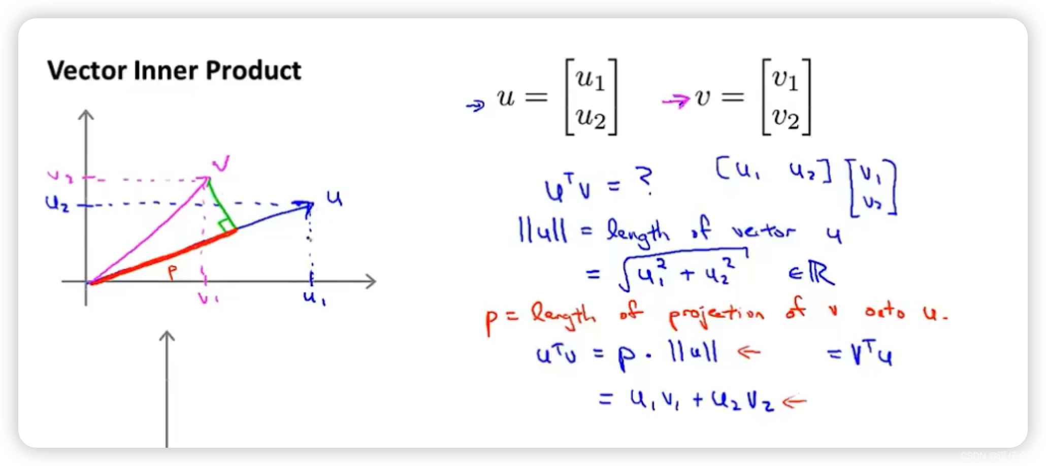
- For two vectors u ⃗ = [ u 1 , u 2 ] T , v ⃗ = [ v 1 , v 2 ] T \vec{u}=[u_1, u_2]^T, \vec{v}=[v_1,v_2]^T u=[u1,u2]T,v=[v1,v2]T
- The dot product of these two vectors can be regarded as v ⃗ \vec{v} v In vector u ⃗ \vec{u} u The projection on the , The length of the projection is p p p, u ⃗ \vec{u} u The length of can be expressed as ∣ ∣ u ∣ ∣ ||u|| ∣∣u∣∣ So the dot product of two vectors can be expressed as : u ⃗ ⋅ v ⃗ = p ⋅ ∣ ∣ u ∣ ∣ = u 1 v 1 + u 2 v 2 \vec{u} \cdot \vec{v}=p\cdot ||u|| = u_1v_1 + u_2v_2 u⋅v=p⋅∣∣u∣∣=u1v1+u2v2
According to the preliminary knowledge of dot product , To achieve m i n θ 1 2 Σ j = 1 n θ j 2 min_\theta\frac{1}{2}\Sigma_{j=1}^n\theta_j^2 minθ21Σj=1nθj2 amount to m i n θ 1 2 Σ j = 1 n ∣ ∣ θ j ∣ ∣ 2 min_\theta\frac{1}{2}\Sigma_{j=1}^n||\theta_j||^2 minθ21Σj=1n∣∣θj∣∣2 And the original constraints :
θ T x > = 1 , i f y i = 1 \theta^Tx>=1, ~~if~~ y_i=1 θTx>=1, if yi=1
θ T x < = − 1 , i f y i = 0 \theta^Tx<=-1, ~~if~~ y_i=0 θTx<=−1, if yi=0
You can write :
p i ⋅ ∣ ∣ θ ∣ ∣ > = 1 , i f y i = 1 p_i\cdot ||\theta|| >=1,~~if~~ y_i=1 pi⋅∣∣θ∣∣>=1, if yi=1
p i ⋅ ∣ ∣ θ ∣ ∣ < = − 1 , i f y i = 0 p_i\cdot ||\theta|| <=-1,~~if~~ y_i=0 pi⋅∣∣θ∣∣<=−1, if yi=0
Why? SVM Don't choose small margin
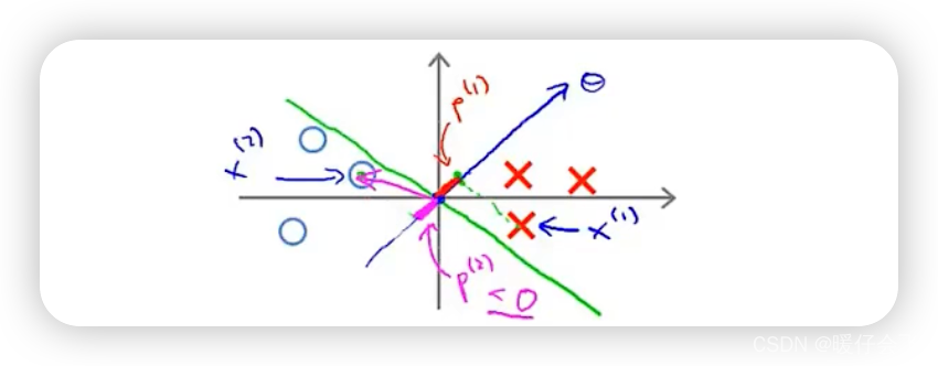
- Suppose there is a pile of points that need to be separated ( Red and blue )
- Suppose there is an optional decision boundary ( Green line ), its margin A very small , Now let's see why SVM Will not choose the decision in this case .
Add a little knowledge , θ T \theta^T θT This vector is perpendicular to the decision boundary . For example, if I have a hyperplane y = − x y=-x y=−x As a decision boundary ( Here, for simplicity, the intercept is temporarily used as 0 0 0 ( θ 0 = 0 \theta_0=0 θ0=0) What if ), y = − x y=-x y=−x You can also write : x + y = 0 x+y=0 x+y=0 So his θ T \theta^T θT The vector is expressed as θ T = [ 1 , 1 ] \theta^T = [1, 1] θT=[1,1];
So to sum up , The decision boundary is a slope of − 1 -1 −1 The straight line of , And the corresponding θ T \theta^T θT The vector does point diagonally to the top right , As shown in the figure below :

- Continue to look at the current situation , According to our existing knowledge of the dot product above , We can get that the loss of the two points closest to the decision boundary can be expressed as :
- p 1 ⋅ ∣ ∣ θ ∣ ∣ p_1\cdot ||\theta|| p1⋅∣∣θ∣∣
- p 2 ⋅ ∣ ∣ θ ∣ ∣ p_2\cdot ||\theta|| p2⋅∣∣θ∣∣
- And because of this margin A very small , Means p 1 p_1 p1 and p 2 p_2 p2 A very small , Don't forget our constraints above :
p i ⋅ ∣ ∣ θ ∣ ∣ > = 1 , i f y i = 1 p_i\cdot ||\theta|| >=1,~~if~~ y_i=1 pi⋅∣∣θ∣∣>=1, if yi=1
p i ⋅ ∣ ∣ θ ∣ ∣ < = − 1 , i f y i = 0 p_i\cdot ||\theta|| <=-1,~~if~~ y_i=0 pi⋅∣∣θ∣∣<=−1, if yi=0 - So if p 1 p_1 p1 and p 2 p_2 p2 A very small , We have to make sure that ∣ ∣ θ ∣ ∣ ||\theta|| ∣∣θ∣∣ Great to meet the results > = 1 >=1 >=1 perhaps < = − 1 <=-1 <=−1 The requirements of
- and ∣ ∣ θ ∣ ∣ ||\theta|| ∣∣θ∣∣ It means violating the optimization goal m i n θ 1 2 Σ j = 1 n θ j 2 min_\theta\frac{1}{2}\Sigma_{j=1}^n\theta_j^2 minθ21Σj=1nθj2
- Therefore, in order not to make the optimization objectives and constraints conflict , We have to ensure that the decision boundary margin The larger . So let's take a look at the right situation , And make corresponding analysis .
When SVM Choose a reasonable margin

-
In this situation , hypothesis margin The straight line can be used x = 0 x=0 x=0 To express ; That is, it can be expressed as x + 0 y = 0 x+0y=0 x+0y=0 So the corresponding vector θ T = [ 1 , 0 ] \theta^T = [1,0] θT=[1,0]
-
At this time, the losses of the two positive and negative samples closest to the decision boundary are :

- p 1 ⋅ ∣ ∣ θ ∣ ∣ p_1\cdot ||\theta|| p1⋅∣∣θ∣∣
- p 2 ⋅ ∣ ∣ θ ∣ ∣ p_2\cdot ||\theta|| p2⋅∣∣θ∣∣
- And because the p 1 p_1 p1, p 1 p_1 p1 Relatively large , therefore θ T \theta^T θT Can guarantee that ∣ ∣ θ ∣ ∣ ||\theta|| ∣∣θ∣∣ The constraints are met in the case of :
p i ⋅ ∣ ∣ θ ∣ ∣ > = 1 , i f y i = 1 p_i\cdot ||\theta|| >=1,~~if~~ y_i=1 pi⋅∣∣θ∣∣>=1, if yi=1
p i ⋅ ∣ ∣ θ ∣ ∣ < = − 1 , i f y i = 0 p_i\cdot ||\theta|| <=-1,~~if~~ y_i=0 pi⋅∣∣θ∣∣<=−1, if yi=0 -
So compare two different SVM Decision boundaries , Because the second can be in ∣ ∣ θ ∣ ∣ ||\theta|| ∣∣θ∣∣ In small cases, the constraints are guaranteed to be established , therefore SVM Will choose the big one margin Classification strategy .
版权声明
本文为[Warm baby can fly]所创,转载请带上原文链接,感谢
https://yzsam.com/2022/04/202204220333411226.html
边栏推荐
- Full summary of 18 tax categories of tax law with memory tips
- Zabbix5 series - making topology map (XIII)
- Docker starts the general solution of three warnings of redis official image
- 7-Zip exposes zero day security vulnerabilities! Provide administrator privileges to attackers by "impersonating file extensions"
- Xampp configuration Xdebug extension, php7 Version 2.2
- Single example of multithreading
- Brief introduction of Bluetooth protocol stack
- Bubble ranking and running for president
- VOS3000 8.05安装及源码
- Redis database
猜你喜欢

GPU深度学习环境配置

Deep learning and image recognition: principle and practice notes day_ ten
![[cloud computing] three virtual machines complete spark yard cluster deployment and write Scala applications to realize word count statistics](/img/97/3bd0c04dd00d56dc35a8742a7aa0ef.png)
[cloud computing] three virtual machines complete spark yard cluster deployment and write Scala applications to realize word count statistics

Vscode shell
百度离线地图研发--laravel框架

Mysql8 hard disk version installation configuration

MongoDB——聚合管道之$project操作
【云计算】3台虚拟机完成Spark Yarn集群部署并编写Scala应用程序实现单词计数统计
GPU deep learning environment configuration

Deep learning and image recognition: principle and practice notes day_ sixteen
随机推荐
Vscode shell
Manual lock implementation of multithreading
Multithreaded deadlock use case
CentOS offline installation of MySQL
【C】 Guess the number, shut down the applet, and practice some branch loops
解决Flutter中ThemeData.primaryColor在AppBar等组件中不生效
College English vocabulary analysis Chinese University MOOC Huazhong University of science and technology
Rasa dialogue robot serial 2 lesson 121: the actual operation of Rasa dialogue robot debugging project: the whole process demonstration of e-commerce retail dialogue robot operation process debugging-
Use of logical backup MySQL dump in MySQL
Vos3000 8.05 installation and source code
C language constant, string, escape character, initial level of annotation
An article gives you a preliminary understanding of the basic knowledge of C language operators
2021-11-06 database
STL learning
Finition musicale de guitare
Implementation of MySQL dblink and solution of @ problem in password
wangEditor富文本编辑器使用、编辑器内容转json格式
Socket to do a simple network sniffer
The mountain is high and the road is far away, fearing no danger
JDBC uses precompiling to execute DQL statements, and the output is placeholder content. Why?