当前位置:网站首页>Fundamentals of graphics - depth of field / DOF
Fundamentals of graphics - depth of field / DOF
2022-04-22 05:24:00 【Sang Lai 93】
Fundamentals of graphics | Depth of field effect (Depth of Field/DOF)
List of articles
One 、 Preface
The depth of field (DOF) It is a common post-processing effect to simulate the focusing characteristics of camera lens .
in real life , The camera can only focus sharply on objects within a specific distance , Objects closer or farther away from the camera will lose some focus .
Blur not only provides a visual cue about the distance of the object , Out of focus imaging is also introduced (Bokeh, Scattered scenery ).
Bokeh, Also known as Jiao Wai , It's a photographic term , Generally speaking, it is used in photographic imaging with shallow depth of field , Pictures falling outside the depth of field , There will be a gradual effect of loose blur .
Depth of field schematic :

Scattered view diagram :

Two 、 Depth of field effect
2.1 Principles of Physics
The depth of field , It refers to the relatively clear imaging range before and after the focus of the camera . The image within the depth of field is clear , The image before or after this range is blurred .
The simplest form of camera is the perfect pinhole camera , It has an image plane for recording light . Before this plane is a plane called aperture (aperture) A small hole in the wall : Only one beam is allowed to pass through .
Objects in front of the camera emit or reflect light in multiple directions , This produces a lot of light . For each point , Only one ray of light can pass through the hole and be recorded .
Here's the picture , Recorded 3 A little bit .

Because each point produces only one beam , Therefore, the image produced by recording is always sharp .
But a single beam is not bright enough , It takes a long time to accumulate ( This means that the camera needs a long exposure time ) To get a clear image .
To reduce exposure time , Light needs to accumulate fast enough . The only way is to record multiple rays at the same time . This can be achieved by increasing the radius of the aperture .
Suppose the aperture is circular , This means that each point will project a beam on the image plane , Not light . So we will receive more light , But it's no longer a point , It's a disc .
Here's the picture , Use a larger aperture .

To refocus the light , We need to restore the beam to a point , This can be achieved by adding a lens in front of the aperture . The lens can bend light , Refocus . This creates a bright and sharp image , But only in one range .
For distant points , Not enough focus , And for the nearest point , The focus is over again . Both turn the image into a beam , It becomes blurred , And this fuzzy projection is Diffuse circle (circle of confusion), Referred to as CoC.

2.2 Dispersion circle quantization
When the imaging plane is not in focus , The light cannot be focused at one point , It will spread around . The scattered range is called Circle Of Confusion, abbreviation COC.
As shown in the figure , Shows dispersion circles with different radii .

So how to quantify the size of the dispersion circle ?
According to the picture below :

The lens ( The aperture diameter is A A A) And imaging plane position ( The distance between the imaging plane and the aperture is I I I).
At a distance of P P P The point of , Just enough to fall on the imaging plane .
According to the convex lens imaging formula :
1 u + 1 v = 1 F \frac{1}{u} + \frac{1}{v} = \frac{1}{F} u1+v1=F1
among , u u u Indicates the object distance , v v v Indicates the image distance , F F F Indicates the focal length .
Then there are :
1 P + 1 I = 1 F \frac{1}{P} + \frac{1}{I} = \frac{1}{F} P1+I1=F1
At a distance of D D D The object , The imaging plane is formed with a diameter of C C C The dispersion circle , It is focused as a projection point by a convex lens , Suppose its distance from the aperture is X X X.
1 D + 1 X = 1 F \frac{1}{D} + \frac{1}{X} = \frac{1}{F} D1+X1=F1
As shown in the figure below , According to similar triangles, there are :
C A = X − I X \frac{C}{A} = \frac{X-I}{X} AC=XX−I

C = A ⋅ X − I X = A ⋅ D F D − F − P F P − F D F D − F = ∣ A F ( P − D ) D ( P − F ) ∣ \begin{aligned} C &= A \cdot \frac{X-I}{X} \\ &= A \cdot \frac{\frac{DF}{D-F}-\frac{PF}{P-F}}{\frac{DF}{D-F}} \\ &= \left | A \frac{F(P-D)}{D(P-F)} \right | \end{aligned} C=A⋅XX−I=A⋅D−FDFD−FDF−P−FPF=∣∣∣∣AD(P−F)F(P−D)∣∣∣∣
among , The symbols in the figure are :
C C C: Diameter of dispersion circle ;
- In calculation, we usually use CoC Represents the radius of the dispersion circle .
A A A: Aperture diameter ;
F F F: The focal length ;
- The focal length It belongs to the inherent attribute of the lens , Not due to changes in other factors , Is the distance between the focusing position of the parallel light after it enters the lens and the center of the lens .
P P P : Focus position ;
- It refers to a specific object distance , Referring to After determining the position of the lens and imaging plane , There is a position in front of the lens that can be focused on the imaging plane , We call the distance between this position and the center of the lens P P P.
- In the picture Plane in focus Literal translation may be misleading , In fact, the original intention of the picture is to look at it from a spatial point of view , The position that can be focused in front of the lens should be parallel to the lens 、 A plane with a fixed distance , The light reflected from each point on the plane can converge into a point on the imaging plane
D D D: Object distance ;
- The distance between the object and the lens , That is, the position of the object at this distance on the lens COC Diffuse circle .
I I I: Imaging surface distance ;
- The distance between the imaging surface and the lens center .
P P P Can pass I I I and F F F determine , When the lens and imaging plane are determined, it can also be called a constant .
therefore , We got one with C C C As the dependent variable , D D D A function that is an argument , The image of this function ( No absolute value ) That's true :

MaxBgdCoC, Refers to the maximum dispersion circle radius of the background , You can get... From the formula on the left .
In the function image ,z It is the of the above formula D D D, That's the independent variable , The vertical axis is CoC value , You can see in the P spot , The radius of the dispersion circle is 0.
Foreground and background increase with distance , The radius of the dispersion circle increases gradually , A steeper and steeper trend .
thus , We can describe the diffusion range of each point on the whole screen .
This is the basis of our subsequent screen post-processing calculation : Get the point on the screen , as well as Its distance from the camera , Other constants can be adjusted by parameters .( The distance between the imaging surface shall not be less than the focal length , Otherwise you can't focus ).
3、 ... and 、 Depth of field implementation
3.1 Simple implementation of non Physics
This part is relatively simple , The author did not realize .
The simplest implementation is shown in the figure below , Start with the camera position , Divided into three parts according to distance :
- Close range blur ;
- The focus range is clear ;
- Distant blur ;

Render by depth ( Distance ) Judge , In the focus area, it is clear , Otherwise, it will be blurred .
The whole process is divided into three Pass:
- Render the scene to a RenderTarget, As a clear version ;
- Take what you got in the last step RenderTarget Fuzzy processing , obtain BluredRT( Fuzzy version );
- synthesis ! Judge whether it should be blurred according to the distance , If not in focus, draw BluredRT, Otherwise draw RenderTarget.
Example Shader Code :
sampler RenderTarget;
sampler BluredRT;
//  Focus range
float fNearDis;
float fFarDis;
float4 ps_main( float2 TexCoord : TEXCOORD0 ) : COLOR0
{
	float4 color = tex2D( RenderTarget, TexCoord );
	if( color.a > fNearDis && color.a < fFarDis )
		return color;
	else
		return tex2D( BluredRT, TexCoord );
}
The effect is as follows :

It can be seen that , The picture above looks unnatural .
The reason is that DOF The transition at the junction of clarity and fuzziness is too stiff .
Can pass Add two transition zones Implement a simple gradient .

Example Shader Code :
sampler RenderTarget;
sampler BluredRT;
//  Focus range
float fNearDis;
float fFarDis;
float fNearRange;
float fFarRange;
float4 ps_main( float2 TexCoord : TEXCOORD0 ) : COLOR0
{
	float4 sharp = tex2D( RenderTarget, TexCoord );
	float4 blur= tex2D( BluredRT, TexCoord );
   	// sharp.a Stored
	float percent = max(saturate(sharp.a-fNearDis)/fNearRange),saturate((sharp.a-(fFarDis-fFarRange))/fFarRange));
	return lerp( sharp, blur, percent );
}
The effect is as follows :

3.2 Physics based depth of field effect
3.1 Only through Indistinguishable fuzzy operation To achieve depth of field DOF effect , The effect is not so good .
More in line with physical practice , Is based on 2.2 The derived dispersion circle Circle Of Confusion(COC), Spread the pixel value of a point evenly along the dispersion circle .
But in GPU It is very difficult to achieve outward diffusion in .
thus , This process is usually reversed , When calculating the color of a pixel , According to the size of the dispersion circle of the surrounding pixels, collect from the surrounding pixels (gather) Pixel color .
Blizzard is in Siggraph2014 Shared their Scatter As Gather Method .

The process of collecting , Is in the surrounding pixels , Look for pixels within the surrounding pixel dispersion circle , Accumulate the color according to a certain weight .
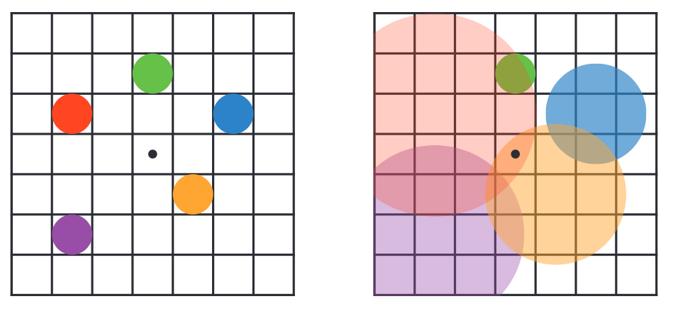
As shown in the figure :
-
On the left , Five points : Red and blue are close , Yellow and purple dots are in the distance , The green dot is the right focus .
-
On the right , The dispersion circle range of each pixel is shown , The larger the scope of the dispersion circle , The smaller the impact on other pixels , The position of the black dot in the middle is affected by two diffusion rings .
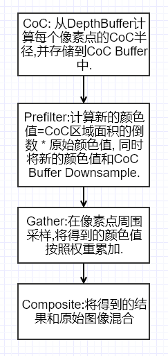
The whole process of depth of field post-processing is roughly like this :
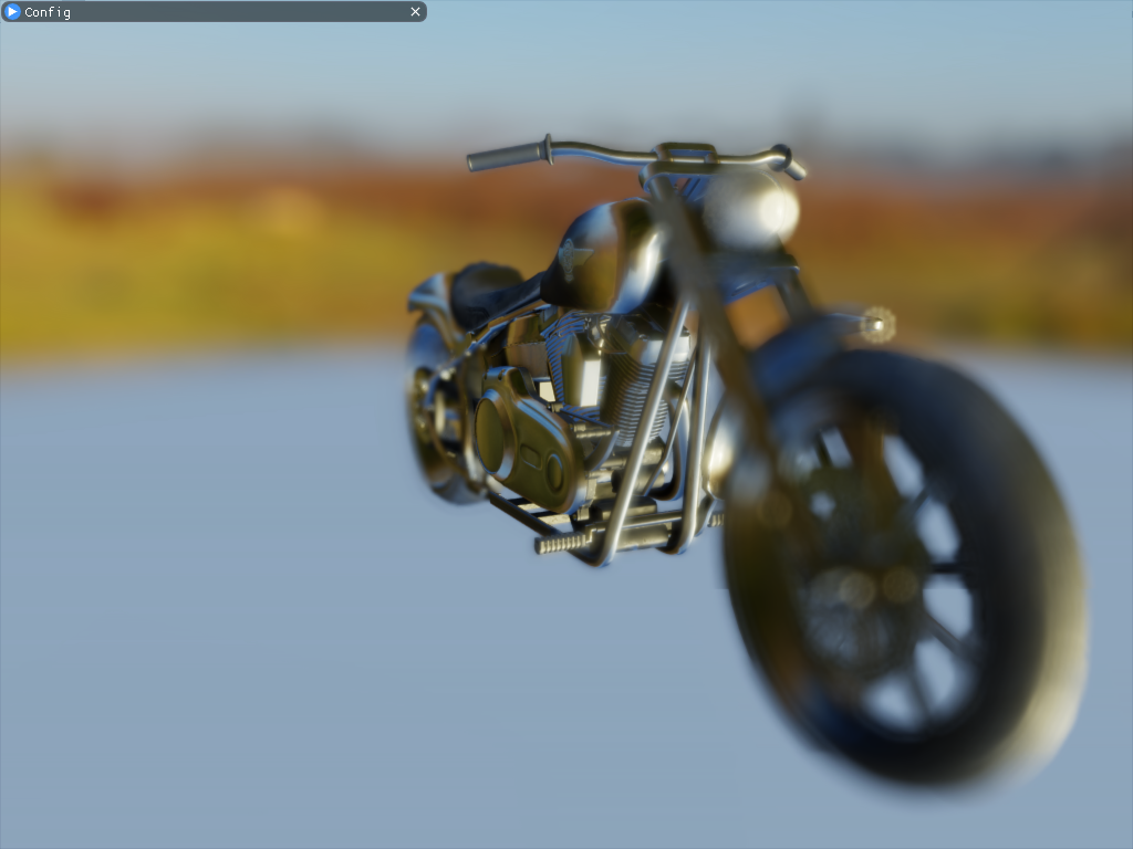
I refer to Unity-Technologies/PostProcessing/DepthOfField and CatlikeCoding-DOF Implement a slightly physics based depth of field DOF effect .
First, the effect diagram of the implementation is given :
The author's implementation is divided into 5 individual Pass, Respectively :
- CoC( Dispersion circle calculation );
- DownSample and Prefilter( Down sampling and pre filtering );
- Bokeh Filter( Scatter filtering );
- Postfilter( Post filtering );
- Combine( blend );
Implementation is based on DX12 Of ComputeShader.
3.2.1 CoC Calculation
For the sake of simplicity and convenience ,CoC There is no choice in the formula 2.2 The formula introduced in . The following method is adopted .
Based on a focus distance (FoucusDistance) A simple focus area (FoucusRange):
just as CatlikeCoding-DOF Used in :

CoC The value adopts the following formula :
c o c = S c e n e D e p t h − F o u c u s D i s t a n c e F o u c u s R a n g e coc = \frac{SceneDepth - FoucusDistance}{FoucusRange} coc=FoucusRangeSceneDepth−FoucusDistance
among , S c e n e D e p t h SceneDepth SceneDepth Represents the depth of pixels in camera space .
As shown in the figure below , The horizontal axis represents the change in depth , The vertical axis means Coc Quantized value of ( Here we truncate it to -1 To 1 Between the value of the ).

Concrete Shader The code is as follows :
RWTexture2D<float>  CoCBuffer               : register(u0);
Texture2D<float>    DepthBuffer             : register(t0);

cbuffer CB0 : register(b0)
{
    float   FoucusDistance;
    float   FoucusRange;
    float2  ClipSpaceNearFar;
};

[numthreads(8, 8, 1)]
void cs_FragCoC
(
    uint3 DTid  : SV_DispatchThreadID
)
{
    // screenPos
    const uint2 ScreenST = DTid.xy;
    // non-linear depth
    float Depth = DepthBuffer[ScreenST];
    //  Go to the depth of camera space
    float SceneDepth = LinearEyeDepth(Depth, ClipSpaceNearFar.x, ClipSpaceNearFar.y);

    // compute simple coc
    float coc = (SceneDepth - FoucusDistance) / FoucusRange;
    coc = clamp(-1, 1, coc);
    //  take [-1,1] Convert to [0,1]
    CoCBuffer[ScreenST] = saturate(coc * 0.5f + 0.5f);
}
3.2.2 Down sampling and pre filtering
We will create the effect of scatter in the case of half resolution . So we need a down sampling Pass.
In this Pass in , We will get the most significant of the adjacent tetrastrians CoC value , Instead of averaging ( It doesn't make sense ).\
For color , Based on brightness and coc Weighting of absolute values .
Last , Four channels of output rgb The color value after down sampling filtering is stored ,alpha The channel stores coc value .
Be careful , there coc The value is multiplied by BokehRadius( Scatter radius ), Convert to scatter distance value .

Concrete Shader The code is as follows :
RWTexture2D<float4> PrefilterColor		: register(u0);
Texture2D<float3>	SceneColor			: register(t0);
Texture2D<float>	CoCBuffer			: register(t1);

SamplerState LinearSampler : register(s0);

cbuffer CB0 : register(b0)
{
    float   BokehRadius;
};

void GetSampleUV(uint2 ScreenCoord, inout float2 UV, inout float2 HalfPixelSize)
{
    float2 ScreenSize;
    PrefilterColor.GetDimensions(ScreenSize.x, ScreenSize.y);
    float2 InvScreenSize = rcp(ScreenSize);
    HalfPixelSize = 0.5 * InvScreenSize;
    UV = ScreenCoord * InvScreenSize + HalfPixelSize;
}

[numthreads(8, 8, 1)]
void cs_FragPrefilter(uint3 DTid : SV_DispatchThreadID)
{
    float2 HalfPixelSize, UV;
    GetSampleUV(DTid.xy, UV, HalfPixelSize);

    // screenPos
    float2 uv0 = UV - HalfPixelSize;
    float2 uv1 = UV + HalfPixelSize;
    float2 uv2 = UV + float2(HalfPixelSize.x, -HalfPixelSize.y);
    float2 uv3 = UV + float2(-HalfPixelSize.x, HalfPixelSize.y);

    // Sample source colors
    float3 c0 = SceneColor.SampleLevel(LinearSampler, uv0, 0).xyz;
    float3 c1 = SceneColor.SampleLevel(LinearSampler, uv1, 0).xyz;
    float3 c2 = SceneColor.SampleLevel(LinearSampler, uv2, 0).xyz;
    float3 c3 = SceneColor.SampleLevel(LinearSampler, uv3, 0).xyz;

    float3 result = (c0 + c1 + c2 + c3) * 0.25;

    // Sample CoCs
    // convert [0,1] to [-1,1]
    float coc0 = CoCBuffer.SampleLevel(LinearSampler, uv0, 0).r * 2 - 1;
    float coc1 = CoCBuffer.SampleLevel(LinearSampler, uv1, 0).r * 2 - 1;
    float coc2 = CoCBuffer.SampleLevel(LinearSampler, uv2, 0).r * 2 - 1;
    float coc3 = CoCBuffer.SampleLevel(LinearSampler, uv3, 0).r * 2 - 1;

    // Apply CoC and luma weights to reduce bleeding and flickering
    float w0 = abs(coc0) / (Max3(c0.r, c0.g, c0.b) + 1.0);
    float w1 = abs(coc1) / (Max3(c1.r, c1.g, c1.b) + 1.0);
    float w2 = abs(coc2) / (Max3(c2.r, c2.g, c2.b) + 1.0);
    float w3 = abs(coc3) / (Max3(c3.r, c3.g, c3.b) + 1.0);

    // Weighted average of the color samples
    half3 avg = c0 * w0 + c1 * w1 + c2 * w2 + c3 * w3;
    avg /= max(w0 + w1 + w2 + w3, 1e-4);

    // Select the largest CoC value
    float cocMin = min(min(min(coc0, coc1), coc2), coc3);
    float cocMax = max(max(max(coc0, coc1), coc2), coc3);
    float coc = (-cocMin >= cocMax ? cocMin : cocMax) * BokehRadius;

    // Premultiply CoC again
    avg *= smoothstep(0, HalfPixelSize.y * 4, abs(coc));

    // alpha The channel stores coc value
    PrefilterColor[DTid.xy] = float4(avg, coc);
}
3.2.3 Scatter filtering
After half resolution pre filtering , We need to create a scatter chart . The method used is the one introduced earlier Gather Methods .
Sample by disc (DiskKernel) To view the Coc Whether the current center point is overwritten .
And accumulate front scattered scenes and back scattered scenes respectively .
Disk sampling provides several , Different number of samples , The rings formed are different .
I choose here KERNEL_LARGE.
#if defined(KERNEL_LARGE)
// rings = 4
// points per ring = 7
static const int kSampleCount = 43;
static const float2 kDiskKernel[kSampleCount] = {
    float2(0,0),
    float2(0.36363637,0),
    float2(0.22672357,0.28430238),
    float2(-0.08091671,0.35451925),
    float2(-0.32762504,0.15777594),
    float2(-0.32762504,-0.15777591),
    float2(-0.08091656,-0.35451928),
    float2(0.22672352,-0.2843024),
    float2(0.6818182,0),
    float2(0.614297,0.29582983),
    float2(0.42510667,0.5330669),
    float2(0.15171885,0.6647236),
    float2(-0.15171883,0.6647236),
    float2(-0.4251068,0.53306687),
    float2(-0.614297,0.29582986),
    float2(-0.6818182,0),
    float2(-0.614297,-0.29582983),
    float2(-0.42510656,-0.53306705),
    float2(-0.15171856,-0.66472363),
    float2(0.1517192,-0.6647235),
    float2(0.4251066,-0.53306705),
    float2(0.614297,-0.29582983),
    float2(1,0),
    float2(0.9555728,0.2947552),
    float2(0.82623875,0.5633201),
    float2(0.6234898,0.7818315),
    float2(0.36534098,0.93087375),
    float2(0.07473,0.9972038),
    float2(-0.22252095,0.9749279),
    float2(-0.50000006,0.8660254),
    float2(-0.73305196,0.6801727),
    float2(-0.90096885,0.43388382),
    float2(-0.98883086,0.14904208),
    float2(-0.9888308,-0.14904249),
    float2(-0.90096885,-0.43388376),
    float2(-0.73305184,-0.6801728),
    float2(-0.4999999,-0.86602545),
    float2(-0.222521,-0.9749279),
    float2(0.07473029,-0.99720377),
    float2(0.36534148,-0.9308736),
    float2(0.6234897,-0.7818316),
    float2(0.8262388,-0.56332),
    float2(0.9555729,-0.29475483),
};

#endif
Concrete Shader The code is as follows :
#define KERNEL_LARGE
#include "DiskKernels.hlsl"
RWTexture2D<float4> BokehColor			: register(u0);
Texture2D<float4>	PrefilterColor		: register(t0);

SamplerState LinearSampler : register(s0);

cbuffer CB0 : register(b0)
{
    float  BokehRadius;
};

//------------------------------------------------------- HELP FUNCTIONS

void GetSampleUV(uint2 ScreenCoord, inout float2 UV, inout float2 PixelSize)
{
    float2 ScreenSize;
    BokehColor.GetDimensions(ScreenSize.x, ScreenSize.y);
    float2 InvScreenSize = rcp(ScreenSize);
    PixelSize = InvScreenSize;
    UV = ScreenCoord * InvScreenSize + 0.5 * InvScreenSize;
}

//------------------------------------------------------- ENTRY POINT
// Bokeh filter with disk-shaped kernels

[numthreads(8, 8, 1)]
void cs_FragBokehFilter(uint3 DTid : SV_DispatchThreadID)
{
    float2 PixelSize, UV;
    GetSampleUV(DTid.xy, UV, PixelSize);

    float4 center = PrefilterColor.SampleLevel(LinearSampler, UV, 0);

    float4 bgAcc = 0.0; // Background: far field bokeh
    float4 fgAcc = 0.0; // Foreground: near field bokeh
    for (int k = 0; k < kSampleCount; ++k)
    {
        float2 offset = kDiskKernel[k] * BokehRadius;
        float dist = length(offset);
        offset *= PixelSize;
        float4 samp = PrefilterColor.SampleLevel(LinearSampler, UV + offset, 0);

        // BG: Compare CoC of the current sample and the center sample and select smaller one.
        float bgCoC = max(min(center.a, samp.a), 0.0);

        // Compare the CoC to the sample distance. Add a small margin to smooth out.
        const float margin = PixelSize.y * 2;
        float bgWeight = saturate((bgCoC - dist + margin) / margin);
        // Foregound's coc is negative
        float fgWeight = saturate((-samp.a - dist + margin) / margin);

        // Cut influence from focused areas because they're darkened by CoC premultiplying. This is only needed for near field.
        //  Reduce the influence of focus area , Their cause CoC Pre multiply and darken . This applies only to the near field .
        fgWeight *= step(PixelSize.y, -samp.a);

        // Accumulation
        bgAcc += half4(samp.rgb, 1.0) * bgWeight;
        fgAcc += half4(samp.rgb, 1.0) * fgWeight;
    }

    // Get the weighted average.
    bgAcc.rgb /= bgAcc.a + (bgAcc.a == 0.0); // zero-div guard
    fgAcc.rgb /= fgAcc.a + (fgAcc.a == 0.0);

    // FG: Normalize the total of the weights.
    //  Normalized foreground scatter weight
    fgAcc.a *= 3.14159265359 / kSampleCount;

    // Alpha premultiplying
    float alpha = saturate(fgAcc.a);
    //  Fusion of front and back scattered scenes
    float3 rgb = lerp(bgAcc.rgb, fgAcc.rgb, alpha);
    // alpha What is stored is the weight of the foreground scatter
    BokehColor[DTid.xy] = float4(rgb, alpha);
}
3.2.4 Post filtering
After creating the scatter effect, add an additional blur pass, This is a post-processing pass. use 3x3 It's called tent filtering (tent filter) Convolution kernel .

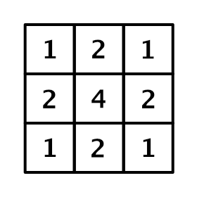
Through a square filter with half moire offset , be based on GPU Bilinear interpolation , Realized a small Gaussian Blur .
Concrete Shader The code is as follows :
RWTexture2D<float4> PostfilterColor		: register(u0);
Texture2D<float4>	BokehColor		    : register(t0);

SamplerState LinearSampler : register(s0);

//------------------------------------------------------- HELP FUNCTIONS
void GetSampleUV(uint2 ScreenCoord, inout float2 UV, inout float2 HalfPixelSize)
{
    float2 ScreenSize;
    PostfilterColor.GetDimensions(ScreenSize.x, ScreenSize.y);
    float2 InvScreenSize = rcp(ScreenSize);
    HalfPixelSize = 0.5 * InvScreenSize;
    UV = ScreenCoord * InvScreenSize + HalfPixelSize;
}

//------------------------------------------------------- ENTRY POINT
// tent filter
/**
*   1 2 1
*   2 4 2
*   1 2 1
*/

[numthreads(8, 8, 1)]
void cs_FragPostfilter(uint3 DTid : SV_DispatchThreadID)
{
    // 9 tap tent filter with 4 bilinear samples
    float2 HalfPixelSize, UV;
    GetSampleUV(DTid.xy, UV, HalfPixelSize);

    float2 uv0 = UV - HalfPixelSize;
    float2 uv1 = UV + HalfPixelSize;
    float2 uv2 = UV + float2(HalfPixelSize.x, -HalfPixelSize.y);
    float2 uv3 = UV + float2(-HalfPixelSize.x, HalfPixelSize.y);

    float4 acc = 0;
    acc += BokehColor.SampleLevel(LinearSampler, uv0, 0);
    acc += BokehColor.SampleLevel(LinearSampler, uv1, 0);
    acc += BokehColor.SampleLevel(LinearSampler, uv2, 0);
    acc += BokehColor.SampleLevel(LinearSampler, uv3, 0);

    PostfilterColor[DTid.xy] = acc / 4.0f;
}
3.2.5 blend
The post filtered scatter image is mixed with the original scene image .
be based on coc Value for nonlinear interpolation .
Concrete Shader The code is as follows :
RWTexture2D<float3> CombineColor		: register(u0);
Texture2D<float3>	TempSceneColor		: register(t0);
Texture2D<float>	CoCBuffer		    : register(t1);
Texture2D<float4>	FilterColor		    : register(t2);

SamplerState LinearSampler : register(s0);

cbuffer CB0 : register(b0)
{
    float  BokehRadius;
};

//------------------------------------------------------- HELP FUNCTIONS
void GetSampleUV(uint2 ScreenCoord, inout float2 UV, inout float2 PixelSize)
{
    float2 ScreenSize;
    CombineColor.GetDimensions(ScreenSize.x, ScreenSize.y);
    float2 InvScreenSize = rcp(ScreenSize);
    PixelSize = InvScreenSize;
    UV = ScreenCoord * InvScreenSize + 0.5 * PixelSize;
}

//------------------------------------------------------- ENTRY POINT
[numthreads(8, 8, 1)]
void cs_FragCombine(uint3 DTid : SV_DispatchThreadID)
{
    // screenPos
    float2 PixelSize, UV;
    GetSampleUV(DTid.xy, UV, PixelSize);
    float3 source = TempSceneColor.SampleLevel(LinearSampler, UV, 0);
    //  Samples the of the current clip CoC value
    float coc = CoCBuffer.SampleLevel(LinearSampler, UV, 0);
    //  Convert to scatter distance
    coc = (coc - 0.5) * 2.0 * BokehRadius;
    //  Sampling scatter
    float4 dof = FilterColor.SampleLevel(LinearSampler, UV, 0);
    // Convert CoC to far field alpha value.
    //  Yes CoC Positive values are interpolated , It is used to obtain the rear scattered view
    float ffa = smoothstep(PixelSize.y * 2.0, PixelSize.y * 4.0, coc);
    //  Nonlinear interpolation
    float3 color = lerp(source, dof.rgb, ffa + dof.a - ffa * dof.a);
    CombineColor[DTid.xy] = color;
}
Refer to the post
- Physics based depth of field effect
- DOF The improved algorithm
- Depth of field in rendering (Depth of Field/DOF)
- CatlikeCoding-DOF
- Depth of field effect ( translate )
- Unity-DOF-Shader
- UE4 Depth of field post-processing effect learning notes ( One ) The basic principle
- UE4 Depth of field post-processing effect learning notes ( Two ) Effect of implementation
版权声明
本文为[Sang Lai 93]所创,转载请带上原文链接,感谢
https://yzsam.com/2022/04/202204210619321842.html
边栏推荐
- Access denied for user ‘root‘@‘% mysql在问题(解决)
- Unity is limited to execute every few frames in update
- Query result processing
- IO stream
- 13.9.1-PointersOnC-20220421
- [WPF] use ellipse or rectangle to make circular progress bar
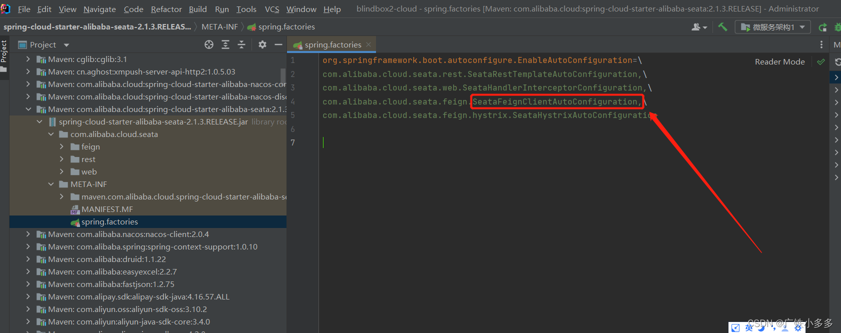
- Feign calls the service, and the called service Seata transaction is not opened or XID is empty
- Detailed explanation of ten functional features of ETL's kettle tool
- Unity button long press detection
- Usage of swagger and common annotation explanation
猜你喜欢

Drawing scatter diagram with MATLAB

Mysql database for the 11th time

PyTorch搭建双向LSTM实现时间序列预测(负荷预测)

Leetcode 1423. Maximum points you can obtain from cards

Strategy mode (2.28-3.6)
Feign calls the service, and the called service Seata transaction is not opened or XID is empty

(2022.1.31-2022.2.14) template mode analysis

Stack (C language)
![[redis notes] data structure and object: Dictionary](/img/0a/0c78c1f897f3a397a87ebb5f138107.png)
[redis notes] data structure and object: Dictionary

Event system for ugui source code analysis in unity (9) - input module (2)
随机推荐
Codeforces Round #781 (Div. 2) ABCD
Pyqt5 + yolov5 + MSS to realize a real-time desktop detection software
数据库(二)MySQL表的增删改查(基础)
Auto.js 画布设置防锯齿paint.setAntiAlias(true);
Codeforces round 783 (Div. 2) d - optimal partition (DP / weight segment tree 2100)
有限单元法基本原理和数值方法_有限元法基本原理
[network protocol] why learn network protocol
萌新看过来 | WeDataSphere 开源社区志愿者招募
unity接入ILRuntime之后 热更工程应用Packages下面的包方法 例如Unity.RenderPipelines.Core.Runtime包
Codeforces Round #783 (Div. 2) D - Optimal Partition(dp/权值线段树 2100)
2022-4-20 operation
Socket communication between server and client
Usage of swagger and common annotation explanation
Typescript function generics
Temporary data node usage based on unitygameframework framework
Feign calls the service, and the called service Seata transaction is not opened or XID is empty
[WPF] cascaded combobox
[candelastudio edit CDD] - 2.3 - realize the jump between multiple securitylevels of $27 service (UDS diagnosis)
Codeforces Round #784 (Div. 4) All Problems
IO流..