当前位置:网站首页>Tensorflow case 4: MNIST handwritten numeral recognition (linear neural network) and its limitations
Tensorflow case 4: MNIST handwritten numeral recognition (linear neural network) and its limitations
2022-04-21 07:11:00 【Kungs8】
Learning goals
- The goal is
- application matmul Realize the calculation of the whole connection layer
- Explain the calculation of accuracy
- application softmax_cross_entropy_with_logits Realization softamx And cross entropy loss calculation
- Explain the role of full connection layer in neural network
- Image recognition is realized by fully connected neural network
- application
- Mnist Handwritten numeral recognition
1、 Data set introduction

The document states :
- train-images-idx3-ubyte.gz: training set images (9912422 bytes)
- train-labels-idx1-ubyte.gz: training set labels (28881 bytes)
- t10k-images-idx3-ubyte.gz: test set images (1648877 bytes)
- t10k-labels-idx1-ubyte.gz: test set labels (4542 bytes)
website :http://yann.lecun.com/exdb/mnist/
1.1 The eigenvalue


1.2 The target

1.3 Get interface
TensorFlow The framework comes with its own interface to obtain this data set , So you don't need to read it yourself .
- from tensorflow.examples.tutorials.mnist import input_data
- mnist = input_data.read_data_sets(FLAGS.data_dir, one_hot=True)
- mnist.train.next_batch(100)( Provide batch acquisition function )
- mnist.train.images、labels
- mnist.test.images、labels
- mnist = input_data.read_data_sets(FLAGS.data_dir, one_hot=True)
2、 actual combat :Mnist Handwritten digit recognition
2.1 Network design
We take only one layer , The last output layer is the neural network . Also known as full connection (full connected) Layer neural networks .

2.1.1 Full connection layer calculation
- tf.matmul(a, b,name=None)+bias
- return: Full connection results , For cross loss calculation
2.2 technological process
1、 Prepare the data
2、 Full connection result calculation
3、 Loss optimization
4、 Model to evaluate ( Calculation accuracy )
mnist = input_data.read_data_sets("./data/mnist/input_data/", one_hot=True)

    # 1、 Prepare the data
    # x [None, 784] y_true [None. 10]
    with tf.variable_scope("mnist_data"):

        x = tf.placeholder(tf.float32, [None, 784])

        y_true = tf.placeholder(tf.int32, [None, 10])

    # 2、 Full connection layer neural network computing
    #  Category :10 Categories    Fully connected layer :10 Neurons
    #  Parameters w: [784, 10]   b:[10]
    #  The calculation formula of full connection layer neural network :[None, 784] * [784, 10] + [10] = [None, 10]
    #  Randomly initialize the weight bias parameter , These are the optimized parameters , You have to use variables op To define
    with tf.variable_scope("fc_model"):
        weight = tf.Variable(tf.random_normal([784, 10], mean=0.0, stddev=1.0), name="w")

        bias = tf.Variable(tf.random_normal([10], mean=0.0, stddev=1.0), name="b")

        # fc Layer calculation
        # y_predict [None, 10] Output results , Provide to softmax Use
        y_predict = tf.matmul(x, weight) + bias

    # 3、softmax Regression and cross entropy loss calculation
    with tf.variable_scope("softmax_crossentropy"):

        # labels: True value  [None, 10]  one_hot
        # logits: Full face output [None,10]
        #  Returns a list of loss components for each sample
        loss = tf.reduce_mean(tf.nn.softmax_cross_entropy_with_logits(labels=y_true,
                                                                      logits=y_predict))

    # 4、 Gradient descent loss optimization
    with tf.variable_scope("optimizer"):

        #  Learning rate
        train_op = tf.train.GradientDescentOptimizer(0.1).minimize(loss)
2.3 Improve the model function
- 1、 Increase the accuracy of calculation
- 2、 Add variables tensorboard Show
- 3、 Add model saving and loading
- 4、 Increase the output of model prediction results
2.3.1 How to calculate the accuracy

- equal_list = tf.equal(tf.argmax(y, 1), tf.argmax(y_label, 1))
- accuracy = tf.reduce_mean(tf.cast(equal_list, tf.float32))
Complete code
# -*- coding=utf-8 -*-
import os
# os.environ["TF_CPP_MIN_LOG_LEVEL"]='1' #  This is the default display level , Show all information
# os.environ["TF_CPP_MIN_LOG_LEVEL"]='2' #  Display only  warning  and  Error
# os.environ["TF_CPP_MIN_LOG_LEVEL"]='3' #  Display only  Error
import time

import tensorflow as tf

from tensorflow.examples.tutorials.mnist import input_data

#  Define whether to train / The sign of prediction
tf.app.flags.DEFINE_integer("is_train", 1, " Training or forecast ")
#  Training steps
tf.app.flags.DEFINE_integer("train_step", 0, " The steps of the training model ")
#  Define the path of the model
tf.app.flags.DEFINE_string("model_dir", " ", " The path of model preservation + Model name ")
FLAGS = tf.app.flags.FLAGS


#  The operation method of this model terminal
# python3 day02_05nn_mnist_FullDemo.py --is_train=1 --train_step=2000  #  Training
# python3 day02_05nn_mnist_FullDemo.py --is_train=0  #  forecast

# tensorboard  Terminal view
# tensorboard --logdir="./temp/summary/"


def full_connected_nn():
    """
     Full connection layer neural network Mnist Handwritten numeral recognition training
    :return:
    """
    mnist = input_data.read_data_sets("../data/mnist/input_data", one_hot=True)

    # 1、 Get data , Define eigenvalue and target tensor
    with tf.variable_scope("data"):
        #  Define a placeholder for the characteristic value
        x = tf.placeholder(tf.float32, [None, 784], name="feature")

        #  Define the target value placeholder
        y_true = tf.placeholder(tf.int32, [None, 10], name="label")

    # 2、 According to the number of categories identified 、 Establish a full connection layer network
    #  Handwritten numerals 10 Categories
    #  A layer of neural network is designed , The last layer ,10 Neurons
    #  Determine the parameters of the network weight [784, 10], bias [10]
    #  To perform the matrix operation of the whole connection layer  [None, 784] * [784, 10] + [10] = [None, 10]
    with tf.variable_scope("fc_model"):
        #  Randomly initialize weights and bias parameters , To use variables OP  Definition
        weights = tf.Variable(tf.random_normal([784, 10], mean=0, stddev=0.1), name="weights")
        bias = tf.Variable(tf.random_normal([10], mean=0, stddev=1.0), name="bias")

        #  Full connection layer operation   10 Neurons   y_predict=[None, 10]
        y_predict = tf.matmul(x, weights) + bias

    # 3、 Based on the output results and the real results softmax、 Calculation of cross entropy loss
    with tf.variable_scope("soft_cross"):
        #  First, calculate the probability of the value output by the network softmax, Then calculate the cross entropy loss
        all_loss = tf.nn.softmax_cross_entropy_with_logits(labels=y_true, logits=y_predict, name="compute_loss")

        #  Find the average loss
        loss = tf.reduce_mean(all_loss)

    # 4、 Define gradient descent optimizer for optimization
    with tf.variable_scope("GD"):
        train_op = tf.train.GradientDescentOptimizer(0.1).minimize(loss)

    # 5、 The accuracy of each training is
    with tf.variable_scope("accuracy"):
        #  Find a list of whether each sample is equal
        equal_list = tf.equal(tf.argmax(y_true, 1), tf.argmax(y_predict, 1))

        #  Calculate the proportion of equal samples
        accuracy = tf.reduce_mean(tf.cast(equal_list, tf.float32))

    # 6、tensorflowboard Data presented
    # 1) The collection should be in tensorflowboard Observed tensor value
    #  Numerical type   --> scalar  Accuracy rate ,  Loss value
    tf.summary.scalar("loss", loss)
    tf.summary.scalar("accuracy", accuracy)

    #  High dimensional tensor values
    tf.summary.histogram("w", weights)
    tf.summary.histogram("b", bias)

    # 2) Merge variables
    merged = tf.summary.merge_all()

    # 7、 Create a to save the model OP
    saver = tf.train.Saver()

    # 8、 Open a session for training
    with tf.Session() as sess:
        #  Initialize variable OP
        sess.run(tf.global_variables_initializer())

        #  establish tensorboard Of events file
        filte_writer = tf.summary.FileWriter("./temp/summary/", graph=sess.graph)

        # 9、 Load the local model to continue training or use it for prediction test set
        checkoutpoint = tf.train.latest_checkpoint("./temp/model/fc_nn_model")
        #  Determine whether the model exists
        if checkoutpoint:
            saver.restore(sess, checkoutpoint)

        #  Judge whether it's training or prediction
        if FLAGS.is_train == 1:
            #  Cycle training
            # for i in range(FLAGS.train_step):
            for i in range(2000):
                #  For each batch 50 Samples
                mnist_x, mnist_y = mnist.train.next_batch(50)

                #  View the size of the data
                # print(mnist_x.shape)

                _, loss_run, accuracy_run, summary = sess.run([train_op, loss, accuracy, merged],
                                                              feed_dict={x: mnist_x, y_true: mnist_y})

                #  Print the effect of each step of training
                print(" The first {0} Step by step 50 The loss of samples is :{1},  Accuracy rate is :{2}".format(i, loss_run, accuracy_run))

                # 3)  Write the running results to the file
                filte_writer.add_summary(summary, i)

                #  every other 100 Next, save the parameters of the model
                if i % 100 == 0:
                    # saver.save(sess, FLAGS.model_dir)
                    saver.save(sess, save_path="./temp/fc_nn_model/fc_nn_model")
        else:
            #  To make predictions
            #  Import model
            #  Load model , From the model, find out the model code that is consistent with the current training ( The same name OP operation ), Overwrite the original value
            checkoutpoint = tf.train.latest_checkpoint("./temp/fc_nn_model/")
            #  Determine whether the model exists
            if checkoutpoint:
                saver.restore(sess, checkoutpoint)

                #  forecast 100 Samples
                N = 200
                a = 0
                for i in range(N):
                    image, label = mnist.test.next_batch(1)

                    #  Real picture numbers
                    result_true = tf.argmax(label, 1).eval()

                    #  The number predicted by neural network
                    result_predict = tf.argmax(sess.run(y_predict, feed_dict={x: image, y_true: label}), 1).eval()

                    #  Directly run the output prediction results of the network
                    print(" The first {0} sample , The real picture number is :{1},  The number predicted by neural network is :{2}".format(
                        i,
                        result_true,
                        result_predict)
                    )
                    if result_true == result_predict:
                        a += 1

                test_accuracy = (a / N) * 100

                print(" Test accuracy :", test_accuracy, "%")
            else:
                print(" The model does not exist ,checkoutpoint  Please output the correct model path ")

    return None


if __name__ == '__main__':
    start_time = time.time()
    full_connected_nn()
    end_time = time.time()
    all_time = end_time - start_time
    print("time:{:.2f} s" .format (all_time))
3、 Limitations of linear neural networks
There is no difference between neural networks with any number of hidden layers and single-layer neural networks , And it's all linear , Moreover, the problems that can be solved by linear model are also limited
1、 More complex abstract data
A single hidden layer has more neurons , You can capture more features . And there are more hidden layers , It means you can extract more complex structures from the data set .

1.1 Increase network depth

1.2 Use the nonlinear activation function

2、 More features of neural networks
2.1 Black box features
- Increasing the depth of the network can really achieve the effect , But how much more ? This is an uncertain question , Or it can change some characteristics of neurons , Change the structure and increase the network depth at the same time , Many of these structures have been tried .
- I don't know what's going on with each neuron inside the network
2.2 More development
More neurons + Deeper networks = More complex abstractions . This is also how simple neurons become smarter , And in the image recognition 、 The reason why go performs so well on these specific issues .
2.2.1 Introduction to neural network expansion
- Types of neural networks
- Basic neural networks : Linear neural networks ,BP neural network ,Hopfield Neural network and so on
- Advanced neural networks : Boltzmann machine , Limited Boltzmann machine , Recurrent neural networks, etc
- Deep neural network : Deep confidence network , Convolutional neural networks , Cyclic neural network ,LSTM Network, etc

Inception: An image recognition model disclosed by Google
2.3 Two challenges : Computing power and training data
In this article , We see some TensorFolw Playground The demonstration explains the mechanism and ability of neural network . As you can see , The foundation of this technology is very simple . Each neuron classifies only one data point into one of two categories . However , By having more neurons and deep layers , A neural network can extract hidden insights and complex patterns in the training data set , And establish an abstract hierarchy .
The next question is , Why isn't everyone using this great technology today ? This is because neural networks still have two major challenges .
- The first is that training deep neural networks requires a lot of computational power .
- second , They require a large number of training data sets . A powerful GPU The server may take days 、 Even weeks , To train a deep network using a data set of millions of images .
and , In order to get the best training results , Different network designs and algorithms need to be combined , And do a lot of trial and error . Now , Some researchers use dozens of GPU The server , Even supercomputers for large-scale distributed training . But in the near future , Fully managed distributed training and prediction services —— For example, Google. TensorFlow Cloud machine learning platform —— May solve these problems , Provide you with cloud based services at a reasonable cost CPU and GPU, It is also possible to open the capabilities of large or deep neural networks to everyone .
版权声明
本文为[Kungs8]所创,转载请带上原文链接,感谢
https://yzsam.com/2022/04/202204210611325747.html
边栏推荐
猜你喜欢
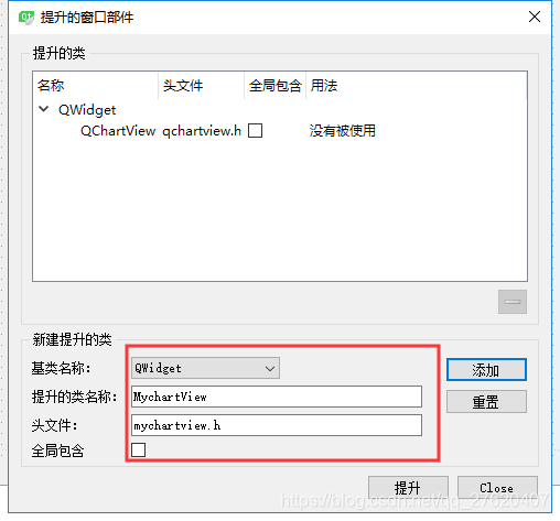
将QT默认控件提升为自定义控件

【Labview】记录下做Labview项目的一些坑点

2、 Signal filtering > mean filtering and median filtering

canvas 绘制路飞
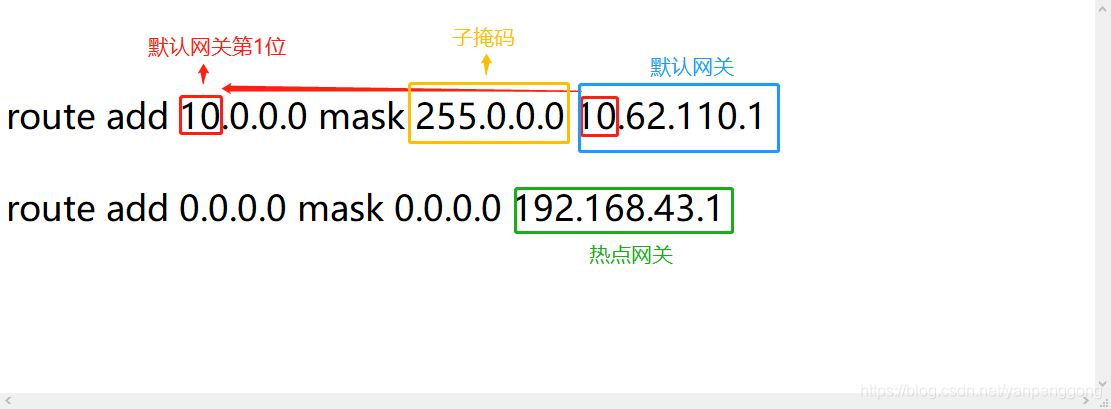
电脑内网外网同时访问-解决办法

ESP32 LVGL8.1 ——msgbox 消息框 (msgbox 28)

【W5500】STM32 H743驱动W5500进行UDP收发

MNIST數據轉化為numpy數組格式的詳細步驟與講解
![3、 3 basic concepts of [Verilog HDL] basic knowledge](/img/5c/ae9d93844c60a0d528a25925dbc464.png)
3、 3 basic concepts of [Verilog HDL] basic knowledge
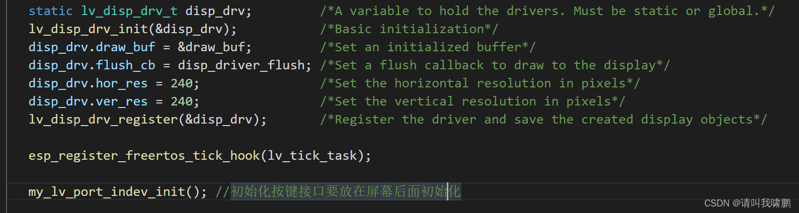
ESP32 LVGL8.1 ——Input devices 输入设备 (Input devices 18)
随机推荐
3-1.pod控制器
logstash 7.x 中时间问题,@timestamp 与本地时间相差 8个小时
每日网安认证测试题(2022年4月14日)
2、 1 [FPGA] initial FPGA
2、 3 [FPGA] how to light the LED
Li Kou video note 21 - depth first search method + 938 question method
3. 事务和视图
Qt中正则表达式的使用
Canvas drawing Luffy
Implementation of prototype networks based on pytorch
ESP32驱动编码器--SIQ-02FVS3 (Vscode + IDF)
Learn SCI paper drawing skills (b)
Neural network reasoning processing of MNIST data set
CISSP认证每日知识点(2022年4月19日)
Draw QQ charts with different distribution
6 service和ingress
每日CISSP认证常错题(2022年4月14日)
CISSP认证每日知识点(2022年4月12日)
ESP32 (UART ECOH)-串口串口回声虫学习(2)
One article will take you to understand the double linked list