Useful link for discrete choice models：https://eml.berkeley.edu/books/choice2.html

Gumbel 分布

Gumbel分布是一种极值型分布, 其The probability density distribution function is
$$f(x;\mu ,\beta )=e^{-z-e^{-z}},z=\frac{x-\mu }{\beta }$$,其中 $\mu$ is the position coefficient （GumbelThe mode of the distribution is $\mu$）; $\beta$ 为尺度系数 (Gumbel分布的方差为 $\frac{{\pi }^2}{6}{\beta }^2$)
标准Gumbel分布,$\mu =0$, $\beta =1$
The probability density distribution function is
$$f(x;\mu ,\beta )=e^{-x-e^{-x}}$$
Python GumbelProbability density function code

import numpy as np
import matplotlib.pyplot as plt
def gumbel_pdf(x, mu=0, beta=1):
    z = (x - mu) / beta
    y = np.exp(-z - np.exp(-z))
    return y
######## 分布函数##############
def gumbel_cdf(x, mu=0, beta=1):
    z = (x - mu) / beta
    y = np.exp(- np.exp(-z))
    return y
################################


x = np.arange(-5., 20, 0.2)
plt.plot(x,gumbel_pdf(x, 0, 1),label= r'$\mu=0,\ \beta=1$')
plt.plot(x,gumbel_pdf(x, 1, 2),label= r'$\mu=1,\ \beta=2$')
plt.axis([-5, 20, 0, 0.4])
plt.ylim([0, 0.5])
plt.xlabel('$x$')
plt.ylabel('Probability')
plt.title('Standard Gumbel distribution probability density distribution curve')
plt.legend(loc='best')
plt.annotate(r'$f(x)=e^{-x-e^{-x}}$',xy=(0, 0.37), xytext=(4.5, 0.45),
             arrowprops=dict(facecolor='black', shrink=0.01,linewidth=0.01),fontsize=14
             )
plt.annotate(r'$f(x)=e^{-\frac{x-\mu}{\beta}-e^{-\frac{x-\mu}{\beta}}}$',xy=(4, 0.2), xytext=(8, 0.1),
             arrowprops=dict(facecolor='black', shrink=0.01,linewidth=0.01),fontsize=16
             )
plt.show()

图片展示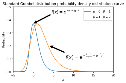

若随机变量 $\xi$ Obey the standardGumbel分布,则其期望为
$$\mathbb{E}(\xi )={\int }_{-\infty }^{+\infty }x{e}^{-x-e^{-x}}dx=-r$$方差为$$\mathbb{D}(\xi )={\int }_{-\infty }^{+\infty }{x}^2{e}^{-x-e^{-x}}dx=\frac{{\pi }^2}{6}$$其中$r$ 为 Euler 常数,$r=0.577215$
The cumulative probability density function formula is
$$F(x;\mu ,\beta )=e^{-e^{-\frac{x-\mu }{\beta }}}$$

matlab Generates a correlation function that follows an extreme value distribution

IType extreme value distribution（Gumbel分布）

If random amount $x$ follow a Weibull distribution（Weibull distribution）,那么 $X=log(x)$ 服从IType extreme value distribution

1. evrnd() Generates extreme value distributed random numbers,The default generation obeys the minimum value extreme value distribution（即Gumbel分布）
   语法

R = evrnd(mu, sigma)%The resulting positional parameter is mu,尺度参数为sigma的随机数
R = evrnd(mu, sigma, m, n,...)
R = evrnd(mu, sigma, [m, n, ...])

2. evpdf(x, mu, sigma) 返回I类型位置参数为mu,尺度参数为sigma在xThe probability density function value of the extreme value distribution at the point

3. evcdf()Used to represent the extreme value cumulative distribution function

p = evcdf(x,mu,sigma)
[p, plo, pup] = evcdf(x, mu, sigma, pcov, alpha)
[p, plo, pup] = evcdf(x, mu,sigma, pcov, alpha, 'upper')

• p = evcdf(x,mu,sigma)返回I类型位置参数为mu,尺度参数为sigma在xThe cumulative probability value of the extreme value distribution at the point
• [p, plo, pup] = evcdf(x, mu, sigma, pcov, alpha)返回I类型位置参数为mu,尺度参数为sigma在xThe confidence interval domain for the cumulative probability value of the extreme value distribution at the point,plo和pupare the upper and lower bounds of the confidence interval domain, respectively
• [p, plo, pup] = evcdf(x, mu,sigma, pcov, alpha, ‘upper’)Returned using an algorithm that more accurately computes the upper tail probabilityI类型位置参数为mu,尺度参数为sigma在xThe confidence interval domain for the cumulative probability value of the extreme value distribution at the point,plo和pupare the upper and lower bounds of the confidence interval domain, respectively

4. evfit() for extreme parameter estimation
   语法

parmhat = evfit(data)
[parmhat,parmci] = evfit(data)
[parmhat,parmci] = evfit(data,alpha)
[...] = evfit(data,alpha,censoring)
[...] = evfit(data,alpha,censoring,freq)
[...] = evfit(data,alpha,censoring,freq,options)

• parmhat = evfit(data)Estimate given sample datadata的服从IMaximum likelihood estimates of parameter values ​​for extreme value-like distributions.The sample data must be a vector of doubles,返回值为ILocation parameter for extreme value-like distributionsmuwith the scale parametersigma
• [parmhat,parmci] = evfit(data) Estimate given sample datadata服从IMaximum likelihood estimates of parameter values ​​for extreme value-like distributions,以及95%Confidence interval for the estimated value of the confidence interval.其中parmciA position parameter representing the estimated parameter valuemuwith the scale parametersigma的区间,The first column is the position parameter interval,The second column is the scale parameter interval.如

[parmhat,parmci] = evfit([1,2,3,4,5,6,7,8])
parmhat =
    5.6400    2.0647
parmci =
    4.1251    1.2050
    7.1549    3.5379

• [parmhat,parmci] = evfit(data,alpha)功能同上,The difference is that you can specify the confidence level yourself.这里的alpha为区间[0,1]A number in the range that specifies the width of the execution interval.默认值为0.05.
• [parmhat,parmci] = evfit(data,alpha,censoring).此处censoringfor the same sample datadataBoolean vector of the same dimension,Censoring for labeling data.其中1Representative data values ​​are right-censored,0Represents data values ​​as exact observations.如

[parmhat,parmci] = evfit([1,2,3,4,5,6,7,8],0.05,[1,0,1,0,1,0,1,0])
parmhat =
 7.0141    1.7707
parmci =
 5.2695    0.8435
 8.7588    3.7173

• [parmhat,parmci] = evfit(data,alpha,censoring,freq)Accepts a frequency vector.其中freqhave the same dimensions as the sample data.通常,The frequency vector contains the integer frequencies of the corresponding elements in the data,But any non-negative value can be in the frequency vector.
• [parmhat,parmci] = evfit(data,alpha,censoring,freq, option)Options can be specified for output.option使用函数statset, 可在matlab控制台help statset

5. evinv() Used to calculate sample values ​​under known probability values

语法

X = evinv(P,mu,sigma)
[X,XLO,XUP] = evinv(P,mu,sigma,pcov,alpha)

6. evlike() Used to compute extreme negative log-likelihoods. matlab help evlike

7. [M,V] = evstat(mu,sigma)The return positional parameter is mu尺度参数为sigma的GumbelThe mean and variance of the distribution.

广义极值分布

GnedenkoIt is proved that the normalized extreme value has a limiting distribution：Gumbel分布、Frechet分布、Weibull分布,are called the first type、Type II and Type III extreme value distributions.JekinsonCombine these three extreme value distributions into one,A generalized extreme value distribution is proposed.若随机变量 $X$ It follows a generalized extreme value distribution,则其概率密度函数为
$$f(x)=\frac{1}{\sigma }[1+\xi (\frac{x-\mu }{\sigma }){]}^{(}-\frac{1}{\xi }-1)exp[1+\xi (\frac{x-\mu }{\sigma }){]}^{-\frac{1}{\xi }}$$其中

• $1+\xi (\frac{x-\mu }{\sigma })>0$
• $\xi$ Indicates that the shape parameter determines the shape of the tails of the distribution
• $-\infty <\mu <\infty$ 为位置参数
• $\sigma >0$是尺度参数.
  当$\xi >0$ 时,The tails of the distribution are longer,趋向于Frechet分布;
  当$\xi =0$ 时,The tails of the distribution are exponential,趋向于Gumbel分布;
  当$\xi <0$ 时,Distributions have finite upper endpoints,趋向于Weibull分布;
  其累积分布函数为
  $$F(x)=exp\{-[1+\xi (\frac{x-\mu }{\sigma }){]}^{-\frac{1}{\xi }}\}$$
  matlabThe related operations are the sameIType extremum distribution prependedg

1. gevrnd() Generates random numbers from a generalized extreme value distribution,Generates a distribution that obeys the maximal extreme value
   语法

R = evrnd(k, mu, sigma)%The resulting shape parameters are k,位置参数为mu,尺度参数为sigma的随机数
R = evrnd(k, mu, sigma, m, n,...)
R = evrnd(k, mu, sigma, [m, n, ...])

附录----数据介绍

完全数据(complete data)： 在研究过程中,The survival time of each study subject was recorded if it could be clearly observed,or the specific time at which the endpoint event occurred,Call this type of data 完全数据.The survival time refers to the time span from the specified observation starting point to the occurrence of a specific end point event.
删失数据（Censoring data）: If at the end of the study,Subjects had other events or survival outcomes outside the study,Survival time to endpoint events could not be recorded definitively,Call this type of data 删失数据,or incomplete data
右删失（right censored） Refers to follow-up observation,The start time of the subject observation is known,但The timing of the endpoint event is unknown,The specific survival time cannot be obtained,Just know that the survival time is greater than the observation time,This type of survival time is called right censoring.Right-censoring is the most common type of data censoring in practical research,Depending on the end time of the observation,可以分为：

• IType censoring
  The observation start time of all subjects was the same,during the study follow-up,Except for subjects who have already experienced an endpoint event,The observation time of the rest of the research subjects was uniformly cut off to a certain fixed time,This type of censoring is IType censoring.IThe censoring time for type censoring is fixed,Therefore, it is also called timing censoring.IType-censoring does not allow individuals to withdraw during the course of the study.
• IIType censoring
  The observation start time of all subjects was the same,在研究的过程中,Follow-up was continued until a sufficient number of end-point outcome events occurred,The study was stopped at this point,The survival time of subjects who did not experience an endpoint event is unknown,This type of censoring is IIType censoring.IIType censoring can be understood as the censoring ratio has been set in advance.
• IIIType censoring
  在实际的研究过程中,There is often no guarantee that all study subjects will enter the study at the same time,after the study started,With the continuous recruitment of research subjects into the study,The observation start time of different research objects is different.同时,before the end of the study,Some study subjects had already experienced endpoint events,Its exact survival time can be recorded,However, some study subjects dropped out of the study,Or at the end of the study still no endpoint event occurred,How long they will live is unclear.
  左删失（right censored）： Suppose that at some point the research subject begins to enter the study for observation,But before that point in time,The time point of interest for the study has occurred,But the exact time could not be specified,This type is known as left-censored data.
  区间删失（right censored）： 在实际的研究中,If continuous observational follow-up is not possible,Only observation time points can be preset,Investigators were only able to know whether each subject had an end-point event between the two follow-up intervals,without knowing the exact time of occurrence,This type of censoring is called interval censoring.

参考文献

【1】Fan Lili,Wang Yanyong,2017. Parameter estimates and instance distributions for generalized extreme value distributions,38(3), 13-17.
【2】Gnedenko B. Sur la distribution limite du terme d’ une serie aleatoire[J], Ann Math, 1943, 44: 423-453.
【3】Jenkinson A F. The frequency distribution of the annual maximum(or minimum) of meteorological elements[J]. The Quarterly Journal of the Royal Meteorological Society, 1955, 81: 158-197.