Kinematic solution of mcnamu wheel

One 、 Mcnamum round Introduction

Read about Robomaster All of my classmates know that ,RM The wheels used in the chariot are mcnamu wheels , This kind of wheel is installed in the same way as ordinary wheels , It can be installed on parallel shafts , But the mcnamu wheel can move in all directions , namely Back and forth movement 、 Move horizontally 、 Rotate around the center . Because of the above advantages , Many industrial omni-directional mobile platforms use this kind of wheel . There are also shortcomings , Just don't wear , It needs to be replaced regularly .

The mcnamu wheel consists of two parts ： Wheel hub and Roller , The hub is the main body of the wheel , The roller is a small ellipsoid like wheel around the wheel hub , The hub and roller have their own shafts , And the included angle between the hub shaft and the roller shaft is 45°（ Can be other angles, but 45° Horns are the most common ）

The installation method of wheat wheel is also exquisite , Although they are all coaxial installation , But unlike ordinary wheels , The wheat wheel is divided into left-handed and right-handed , On a four-wheel chassis, you need to use two left-hand and two right-hand . The installation method is O type , As shown in the figure ：

The picture on the left shows what you see after installation , The figure on the right shows the shape surrounded by rollers with four wheels in contact with the ground , That is to say “O shape ”

there O Shape refers to the shape surrounded by rollers in contact with the ground , Don't ask why the picture on the left looks like X 了

Two 、 Kinematic model of mcnamu wheel

1. Basic knowledge of

1.1 Coordinate system

stay ROS In the robot , The coordinate system is defined with the right hand

about ROS robot , If you take it as the origin of the coordinate system , that

• x Axis ： In front of the
• y Axis ： left side
• z Axis ： upper

As shown in the figure ：

besides , For rotational motion , Also use the right hand to define ：

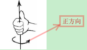
according to The right hand defines , around z The shaft is rotating yes Counter clockwise rotation

1.2 Unit of measurement

ROS Use metric ：

• Linear velocity ：m/s
• angular velocity ：rad/s

1.3 Wheel serial number definition

Left front 1 Right front 2

Back left 3 Right rear 4

2. Inverse kinematics analysis

Inverse kinematics model （inverse kinematic model） The obtained formula can calculate the speed of four wheels according to the motion state of the chassis .

2.1 Decomposition of chassis motion

The motion of a rigid body in a plane can be decomposed into three independent components ：X Shaft translation 、Y Shaft translation 、yaw Shaft rotation . The motion of the chassis can also be divided into three quantities ：

As shown in the figure below :

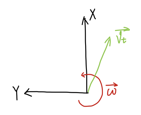
• $v_{tx}$ Express X The speed at which the axis moves , That is, the front and rear direction , Define forward as positive ;
• $v_{ty}$ Express Y The speed at which the axis moves , Right and left , Define left as positive ;
• $\overrightarrow{\omega }$ Express yaw Angular velocity of shaft rotation , Define counterclockwise as positive .

2.2 Calculate the speed of the wheel axis position

As shown in the figure below , Take the right front wheel as an example , The blue box represents the wheel , Define the following variables ：

• $\overrightarrow{r}$ Is the vector from the center of the chassis to the axis of the wheel ;
• $\overrightarrow{v}$ Is the velocity vector of the wheel axis ;
• $\overrightarrow{v_r}$ The axis of the wheel is perpendicular to $\overrightarrow{r}$ The direction of （ The tangent direction ） The velocity component of ;

You can calculate that ：

KaTeX parse error: No such environment: align* at position 8: \begin{̲a̲l̲i̲g̲n̲*̲}̲ \overrightarro…

take $\overrightarrow{r}$ Decompose into $r_x$ and $r_y$, Calculate the wheel axis at X、Y The velocity component of the shaft ：

$$\{\begin{array}{c}{v}_x=v_{tx}+\omega \cdot r_y\\ v_y=v_{ty}+\omega \cdot r_x\end{array}$$

The other three wheels are the same

2.3 Calculate the roller speed in contact with the ground

from 2.2 Calculated wheel axis speed , It can be decomposed into... Along the roller axis $\overrightarrow{v_{\parallel }}$ And perpendicular to the roller axis $\overrightarrow{v_{\perp }}$ , As shown in the figure

among $\overrightarrow{v_{\perp }}$ For idling the roller , You can ignore

Define a unit vector in the direction of the roller $\hat{e}$, For the right front wheel ,$\hat{e}=\frac{1}{\sqrt{2}}\cdot \hat{i}+\frac{1}{\sqrt{2}}\cdot \hat{j}$

Then the velocity along the axis is $\overrightarrow{v}$ stay $\hat{e}$ Projection of direction ：

KaTeX parse error: No such environment: align* at position 8: \begin{̲a̲l̲i̲g̲n̲*̲}̲ \overrightarr…

2.4 Calculate the speed of the wheel （ The linear velocity at the point of contact with the ground ）

As shown in the figure , The wheel speed is $v_w$

Because the roller and the axle are 45° horn , be $v_{\omega }$ Obtainable ：

KaTeX parse error: No such environment: align* at position 8: \begin{̲a̲l̲i̲g̲n̲*̲}̲ v_w&=\frac{v_…

take 2.2 Found $\{\begin{array}{c}{v}_x=v_{tx}+\omega \cdot r_y\\ v_y=v_{ty}+\omega \cdot r_x\end{array}$ Bring it up , The rotational speed of this wheel can be calculated ：
$$v_w=v_{tx}+v_{ty}+\omega (r_x+r_y)$$

Combine the above four steps , The rotational speed of the four wheels can be calculated according to the motion state of the chassis ：

$$\{\begin{array}{c}{v}_{w1}=v_{tx}-v_{ty}-\omega (r_x+r_y)\\ v_{w2}=v_{tx}+v_{ty}+\omega (r_x+r_y)\\ v_{w3}=v_{tx}+v_{ty}-\omega (r_x+r_y)\\ v_{w4}=v_{tx}-v_{ty}+\omega (r_x+r_y)\end{array}$$

The above equations are O Inverse kinematics model of V-shaped wheat wheel chassis .

2.5 Code implementation

// Parameter macro definition 
#define ENCODER_RESOLUTION 1440.0 // Encoder resolution ,  The wheel goes round , The number of pulses generated by the encoder 
#define WHEEL_DIAMETER 0.058 // Wheel diameter , Company ： rice 
#define D_X 0.18 // chassis Y The distance between the centers of the two wheels on the shaft 
#define D_Y 0.25 // chassis X The distance between the centers of the two wheels on the shaft 
#define PID_RATE 50 //PID Adjust the PWM The frequency of the value 

double pulse_per_meter = 0;
float rx_plus_ry_cali = 0.3;
double angular_correction_factor = 1.0;
double linear_correction_factor = 1.0;
double angular_correction_factor = 1.0;

/** * @ Function function ： Kinematics analysis parameter initialization  */
void Kinematics_Init(void)
{
    
	// The wheel goes round , The moving distance is the circumference of the wheel WHEEL_DIAMETER*3.1415926, The pulse signal generated by the encoder is ENCODER_RESOLUTION. Then the pulse signal generated by the motor encoder rotating for one turn can be divided by the circumference of the wheel to get the wheel forward 1m The distance corresponding to the change of encoder count 
    pulse_per_meter = (float)(ENCODER_RESOLUTION/(WHEEL_DIAMETER*3.1415926))/linear_correction_factor;
    
    float r_x = D_X/2;
    float r_y = D_Y/2;
    rx_plus_ry_cali = (r_x + r_y)/angular_correction_factor;
}

/** * @ Function function ： Inverse kinematics analysis , Chassis three-axis speed --> Wheel speed  * @ Input ： Robot three-axis speed  m/s * @ Output ： The target speed that the motor should reach （ One PID During the control cycle , Change of motor encoder count value ） */
void Kinematics_Inverse(int16_t* input, int16_t* output)
{
    
	float v_tx   = (float)input[0];
	float v_ty   = (float)input[1];
	float omega = (float)input[2];
	static float v_w[4] = {
    0};
	
	v_w[0] = v_tx - v_ty - (r_x + r_y)*omega;
	v_w[1] = v_tx + v_ty + (r_x + r_y)*omega;
	v_w[2] = v_tx + v_ty - (r_x + r_y)*omega;
	v_w[3] = v_tx - v_ty + (r_x + r_y)*omega;

    // Calculate a PID During the control cycle , Change of motor encoder count value 
	output[0] = (int16_t)(v_w[0] * pulse_per_meter/PID_RATE);
	output[1] = (int16_t)(v_w[1] * pulse_per_meter/PID_RATE);
	output[2] = (int16_t)(v_w[2] * pulse_per_meter/PID_RATE);
	output[3] = (int16_t)(v_w[3] * pulse_per_meter/PID_RATE);
}

3. Forward kinematics analysis

3.1 Forward kinematics model

Forward kinematics model （forward kinematic model） Let's go through the speed of four wheels , Calculate the motion state of the chassis . It can be solved directly according to the three equations in the inverse kinematics model , such as ：

$$\{\begin{array}{c}{v}_{tx}=\frac{v_4+v_3}{2}\\ v_{ty}=\frac{v_3-v_1}{2}\\ \omega =\frac{v_2-v_3}{2(r_x+r_y)}\end{array}$$

The change of odometer is calculated by integrating the time in the chassis coordinate system

3.2 Code implementation

// Parameter macro definition 
#define ENCODER_MAX 32767 
#define ENCODER_MIN -32768 
#define ENCODER_LOW_WRAP ((ENCODER_MAX - ENCODER_MIN)*0.3+ENCODER_MIN)
#define ENCODER_HIGH_WRAP ((ENCODER_MAX - ENCODER_MIN)*0.7+ENCODER_MIN)
#define PI 3.1415926

// Variable definitions 
int32_t  wheel_turns[4] = {
    0};
int32_t  encoder_sum_current[4] = {
    0};

/** * @ The functionality ： Forward kinematics analysis , Wheel code value -> Chassis three-axis odometer coordinates  * @ Input ： Encoder accumulation value  * @ Output ： Three axis odometer  x y yaw */
void Kinematics_Forward(int16_t* input, int16_t* output)
{
    
	static double dv_w_times_dt[4]; // Instantaneous variation of wheel dxw=dvw*dt
	static double dv_t_times_dt[3]; // Instantaneous change of chassis dxt=dvt*dt
	static int16_t encoder_sum[4];
	
    // Multiply the accumulated value of the left wheel encoder by -1, To calculate the distance forward 
	encoder_sum[0] = -input[0];
	encoder_sum[1] = input[1];
	encoder_sum[2] = -input[2];
	encoder_sum[3] = input[3];
	
	// Encoder count overflow processing 
	for(int i=0;i<4;i++)
	{
    
		if(encoder_sum[i] < ENCODER_LOW_WRAP && encoder_sum_current[i] > ENCODER_HIGH_WRAP)
			wheel_turns[i]++;
		else if(encoder_sum[i] > ENCODER_HIGH_WRAP && encoder_sum_current[i] < ENCODER_LOW_WRAP)
			wheel_turns[i]--;
		else
			wheel_turns[i]=0;
	}

	// Convert the encoder value to the forward distance , Company m
	for(int i=0;i<4;i++)
	{
    	
		dv_w_times_dt[i] = 1.0*(encoder_sum[i] + wheel_turns[i]*(ENCODER_MAX-ENCODER_MIN)-encoder_sum_current[i])/pulse_per_meter;
		encoder_sum_current[i] = encoder_sum[i];
	}
	
    // To calculate the coordinates, so change back 
	dv_w_times_dt[0] = -dv_w_times_dt[0];
	dv_w_times_dt[1] =  dv_w_times_dt[1];
	dv_w_times_dt[2] = -dv_w_times_dt[2];
	dv_w_times_dt[3] =  dv_w_times_dt[3];
	
	// Calculate the chassis coordinate system (base_link) Next x Axis 、y Axis change distance m And Yaw Axis orientation changes rad  The amount of change over time 
	dv_t_times_dt[0] = ( dv_w_times_dt[3] + dv_w_times_dt[2])/2.0;
	dv_t_times_dt[1] = ( dv_w_times_dt[2] - dv_w_times_dt[0])/2.0;
	dv_t_times_dt[2] = ( dv_w_times_dt[1] - dv_w_times_dt[2])/(2*wheel_track_cali);
	
	// Integral calculation odometer coordinate system (odom_frame) The robot under X,Y,Yaw Axis coordinates 
	//dx = ( vx*cos(theta) - vy*sin(theta) )*dt
	//dy = ( vx*sin(theta) + vy*cos(theta) )*dt
	output[0] += (int16_t)(cos((double)output[2])*dv_t_times_dt[0] - sin((double)output[2])*dv_t_times_dt[1]);
	output[1] += (int16_t)(sin((double)output[2])*dv_t_times_dt[0] + cos((double)output[2])*dv_t_times_dt[1]);
	output[2] += (int16_t)(dv_t_times_dt[2]*1000);
		
    //Yaw Axis coordinate change range control -2Π -> 2Π
	if(output[2] > PI)
		output[2] -= 2*PI;
	else if(output[2] < -PI)
		output[2] += 2*PI;
		
	// Send the robot X Axis y Axis Yaw Instantaneous variation of shaft , stay ROS End divided by time 
	output[3] = (int16_t)(dv_t_times_dt[0]);
	output[4] = (int16_t)(dv_t_times_dt[1]);
	output[5] = (int16_t)(dv_t_times_dt[2]);
}

reference ：

【1】https://zhuanlan.zhihu.com/p/20282234

【2】https://blog.csdn.net/shixiaolu63/article/details/78496457