Clean up some previous drafts , I forgot to write and publish half of it , I hope you will forgive me . However, since several people have translated the full text , If you don't understand, you can refer to , This article is really regarded as the ancestor of point cloud generation model . From Stanford , The validation test is really much . It basically tells us that the Gaussian mixture model is easy to use .

1. Summary ：

2018CVPR Conference papers , It's also a pioneer work .
The paper ：http://proceedings.mlr.press/v80/achlioptas18a/achlioptas18a.pdf
Supplementary materials ：http://proceedings.mlr.press/v80/achlioptas18a/achlioptas18a-supp.pdf
Code ：https://github.com/optas/latent_3d_points

Main points of this paper ：

• Study the representation of point cloud , The main use of deep AutoEncoder.

• Different generation models are compared ,l-GAN Much better GMMs：

  The model includes ：
  1）GANs： Act directly on the original point cloud ;
  2）l-GANs（latent-GANs）： Point cloud features directly acting on potential space , use AE First extract the features of potential spatial point cloud ;
  3）GMMs： Gaussian mixture model

  Evaluation methods ：
  1） Sample fidelity ;
  2） Coverage measurement ;

2. Contribution point ：

• A new point cloud AE frame ;
• The first set of point cloud depth generation model ;
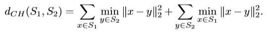
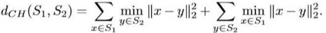
• A new measure of , Based on the best match between two different point cloud sets ;

3. Measurement method ：

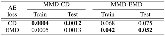
3.1 Measure

1） EMD： Geodesic distance

Limit ： The number of two point sets needs to be consistent , It's a transportation problem between two sets , One-to-one correspondence .
advantage ： It's almost everywhere

2） CD： Nearest neighbor metric

advantage ： Measure the square of the nearest neighbor between one set and another , There is no limit to the number of two sets being the same . And the calculation is EMD More efficient .

3.2 Generate model metrics

1） JSD：

Euclidean three-dimensional boundary distribution of Jensen - Shannon divergence （Jensen-Shannon Divergence ）
Used to measure the similarity between two distributions

2） Converage：

Calculation of coverage ： use B And A To measure . The essence is to calculate the distance to get . So the calculation of similarity still needs to use the basic measurement CD or EMD.
Distance calculation formula at point level ; EMD It's almost everywhere , but CD Differentiable and computationally more efficient ;

1. Earth Mover’s distance（EMD）
   

2. Chamfer（pseudo）distance（CD）
   

3） Minimum matching distance （Minimum Matching Distance,MMD）

MMD Can be measured by A Yes B The fidelity of , make up Disadvantages of coverage （ Cannot accurately indicate Geometry A How well is covered in ）

Compare

MMD And Coverage complementary . stay MMD Small Cov In big cases , Point cloud A The collection was captured with good fidelity B All modes of .
JSD Is to calculate the distribution similarity , Therefore, it is a rough evaluation of the similarity between the two sets .JSD And MMD There is a good correlation , Can be used as an effective alternative .

4. Representation and generation model

Basic block ：
AEs： Recode the input schema . Compressed features can be used $z$ To express the original point cloud . Can be used for reconstruction tasks .

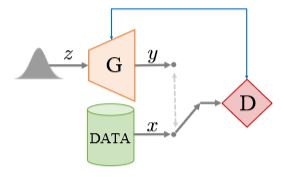
GANs： Infrastructure ： generator G Discriminator D.
G： The generated sample cannot be distinguished from the real data , By putting a simple distribution Randomly selected samples are passed to the generator function .
D： Distinguish the synthetic sample from the actual sample ;

GMM： A probabilistic model , Used to represent a population assuming a multimodal Gaussian distribution , That is, it is composed of multiple sub populations , Each sub population obeys Gaussian distribution . Suppose the number of subpopulations is known , Maximize expectations （EM） The algorithm can learn from random samples GMM Parameters （ In fact, it is the mean and variance of Gaussian distribution ）.

4.1 original GAN Model （r-GAN）：

Training data set ：20483 Point cloud
Judging device ： Structure and AE identical , It's no use Batch-Norm, Use Leaky ReLU, The last full connection layer output is sent to sigmoid Activation function .
generator ： Gaussian noise as input ,5 individual FC-ReLu Layer mapping to 20483 Output

4.2 Hidden space GAN（l-GAN）：

First train a AE, And then use AE The encoder obtains implicit expression features Z.
Both generator and discriminator are based on Z To operate . Optimize implicit expression features Z.
advantage ： Simple structure . say concretely , Single hidden layer MLP Generator with two hidden layers MLP Discriminator coupling , Enough to produce measurable and realistic results .

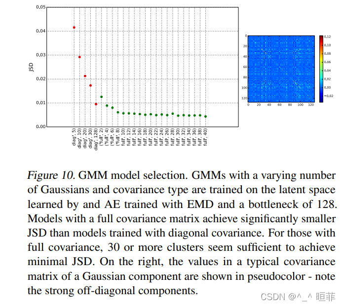
4.3 Gaussian mixture model （GMM）：

stay AE Build a series of Gaussian mixture models in the learning hidden space （GMMs）.
Various quantities of Gaussian components and diagonal or complete covariance matrices are tried .
The distribution is first configured and then sampled AE The decoder of , GMM It can be regarded as a point cloud generator , similar l-GANs.

5. Experimental evaluation

Data sets

ShapeNet： The axis is aligned and centered in the unit sphere . The data is divided into 85%：5%：10% = Training ： verification ： test .
JSD The evaluation uses 283 Regular voxel mesh .

AE The reconstruction

Representativeness
Use AE The effect of editing the part of the point cloud by simple addition algebra in latent space .

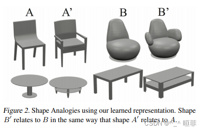
Shape editing ： The formula is as follows , The effect is as follows 3, Reference resources （Yi et al. 2016a）

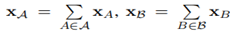
It is assumed that a given category can be further divided into two subclasses ：A And B, The two have structural features that do not exist in each other , Can be represented by their average potential ${\mathbf{X}}_B-{\mathbf{X}}_A$ To simulate the difference between the two subclasses . The same can be done through $x_{A^{\prime }}=x_A+{\mathbf{X}}_B-{\mathbf{X}}_A$. See the figure below 3.

Generalization ： The reconstructed shape is almost as good as the training shape . Use MMD Capture AE The generalization of .

Dive space exploration ： linear interpolation
The implicit expressions of the two shapes are linearly interpolated and the results are decoded , Get an intermediate variant between two shapes （morph-like）.

Shape completion ：

classification ：
Training comes from 55 Of two categories of man-made objects 57,000 A model . Specifically for this experiment , We use 512 The characteristics of dimensions . Using linear SVM To classify , The following table shows the effect . You can see the simplicity AE The effect is good .

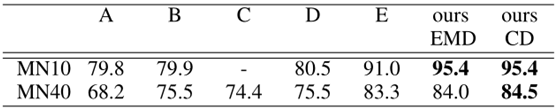
surface 2 ModelNet10 / 40 Classification performance on （％）. Compare A：SPH（Kazhdan wait forsomeone ,2003）,B：LFD（Chen wait forsomeone ,2003）,C：TL-Net（Girdhar wait forsomeone ,2016）,D：VConv-DAE（Sharma wait forsomeone . ,2016）,E：3D-GAN（Wu etc. ,2016）.

there SVM Of the classifier AE Use an encoder , Each layer corresponds to a filter ：128,128,256,512 individual , There were 1024,2048,2048*3 A neuron decoder . Each layer uses BatchNorm. Along the Z Rotate the axis to each batch of input point cloud to realize online data enhancement . Training 1000 The wheel CD Loss and 1100 The wheel EMD. Some parameters of classification are shown in the table below .

Evaluation generation model

The comparison of various methods is shown in the table below , In the verification of - The segmentation passes the minimum JSD choice epochs/ Model , Evaluate on the test segmentation of the chair dataset 5 A generator . We report ：A： Sample based memory baseline ,B：r-GAN,C：1-GAN（AE-CD）,D：1-GAN（AE-EMD）,E：1-WGAN（AE-EMD）, F：GMM（AE-EMD）. You can see GMM The best effect .

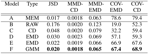
chart 6 It shows that as the training goes on , The generated synthetic data set is based on GAN The model maintains the relationship between test data JSD（ Left ） and MMD And coverage （ Right ）.
Be careful ：r-GAN Strive to provide good coverage and good fidelity of the test set ; This implies a recognized fact , End to end GAN It's usually hard to train .
With less training ,l-GAN (AE-CD) Perform better in fidelity , But coverage is still low . Switch to based on EMD Of AE Used to represent and use the same potential GAN framework （l-GAN,AE-EMD）, Resulting in significant improvements in coverage and fidelity . Two l-GAN Although there are known problems with mode crashes ： Halfway through the training , First, coverage began to decline , But the fidelity is still at a good level , This means that they over fit a small part of the data . later , This was followed by a catastrophic collapse , Coverage dropped to 0.5％. As expected , Switch to potential WGAN This kind of collapse has been largely eliminated .

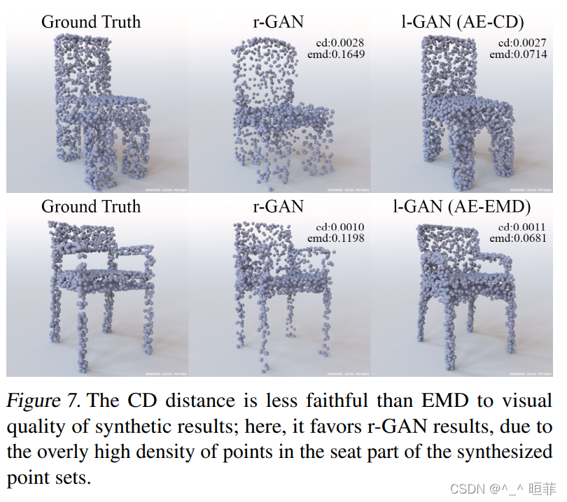
chart 7 Explained CD The blindness of distance , It's very uncomfortable, very discriminative . Only some good matches have additional side effects , That is, coverage CD> coverage EMD When .

6. other

Shape analogy ：

Here through the hidden space Perform linear operation + Euclidean nearest neighbor search Find a similar shape , The Euclidean property of implicit space is proved .
Specifically ： It is known that $A$ ,$A^{\prime }$, and $B$, that $B^{\prime }=B+（A^{\prime }-A）$, That is, searching $B$ Potential space with $B^{\prime }$ The result of nearest neighbor . Can be used to find shape analogies . As shown in the figure below .

Auto coder

Data sets D-FAUST：10 personal , Everyone 14 A sport , Each movement consists of 300 Time series capture of a grid .
This experiment ： Random sampling 80 Grid (s) , Each mesh is extracted 4096 A point cloud . The following figure shows the effect of interpolation .

Parameter selection

See the paper for other detailed parameters

GMM
Conclusion ： The model with complete covariance matrix is better than the model trained with diagonal covariance JSD Much smaller .
Using the complete covariance matrix ,30 One or more clusters seem to be enough to get the smallest JSD.

limited

Chairs with rare shapes will be incorrectly decoded .
AE May miss high-frequency geometric details , You can't rebuild an uncommon example .

7. Reference resources

1. Thesis translation
2. Thesis translation 2