引言

课程视频链接：https://www.bilibili.com/video/BV1Y7411d7Ys?from=search&seid=17942018663670881374
笔者认为讲得十分通俗易懂

1 线性模型

1.1 线性模型

$$\hat{y}=x\ast w+b$$

1.2 损失（针对单个样本）

$$loss=(\hat{y}-y{)}^2=(x\ast w-y{)}^2$$

1.3 均方误差 MSE（针对整个训练样本）

$$cost=\frac{1}{N}\sum _{n=1}^N({\hat{y}}_n-y_n{)}^2$$

1.4 代码实现（用numpy）

import numpy as np
import matplotlib.pyplot as plt
# 数据集准备
x_data = [1.0,2.0,3.0]
y_data = [2.0,4.0,6.0]

def forward(x):  # 定义线性模型
    return x*w

def loss(x,y):  # 定义损失函数（单个样本计算损失）
    y_pred = forward(x)
    return (y_pred - y)*(y_pred - y)

w_list = []
mse_list = []
for w in np.arange(0.0,4.1,0.1):  # 穷举法列举权重
    print('w = ',w)
    l_sum = 0
    for x_val,y_val in zip(x_data,y_data):
        y_pred_val = forward(x_val)
        loss_val = loss(x_val,y_val)
        l_sum+=loss_val
        print('\t',x_val,y_val,y_pred_val,loss_val)
    print('MSE=',l_sum/3)
    w_list.append(w)
    mse_list.append(l_sum/3)
# 绘图
plt.plot(w_list,mse_list)
plt.ylabel('loss')
plt.xlabel('w')
plt.show()

运行结果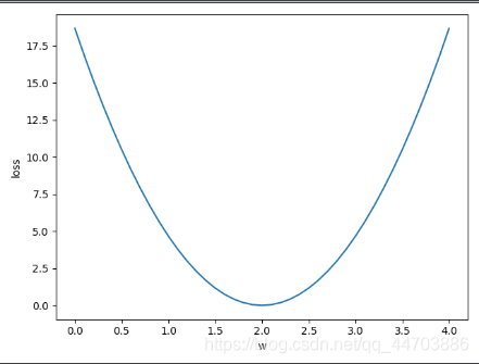

可视化训练过程（Visdom工具）
http://github.com/facebookresearch/visdom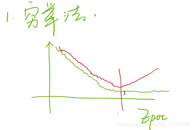

matlab 3d图绘制

2 梯度下降

搜索最佳权重的方法(优化问题)：

• 穷举法
• 分治法（只针对凸函数，否则只能找到局部最优）
• 梯度下降法（贪心）

梯度定义：

$$\begin{gathered} \frac{\partial cost(w)}{\partial w}=\frac{\partial }{\partial w}\frac{1}{N}\sum _{n=1}^N({\hat{y}}_n-y_n{)}^2 \\ =\frac{1}{N}\sum _{n=1}^N\frac{\partial }{\partial w}(x_n\cdot w-y_n{)}^2 \\ =\frac{1}{N}\sum _{n=1}^{N}2\cdot (x_n\cdot w-y_n)\frac{\partial (x_n\cdot w-y_n)}{\partial w} \\ =\frac{1}{N}\sum _{n=1}^{N}2\cdot x_n\cdot (x_n\cdot w-y_n) \end{gathered}$$

2.1 梯度下降算法

$$w=w-\frac{\partial cost}{\partial w}$$
其中
$$\frac{\partial cost}{\partial w}=\frac{1}{N}\sum _{n=1}^{N}2\cdot x_n\cdot (x_n\cdot w-y_n)$$

w = 1.0
def forward(x):  # 线性模型
    return x*w

def cost(xs,ys):
    cost = 0
    for x,y in zip(xs,ys):
        y_pred = forward(x)
        cost += (y_pred-y)**2
        return cost/len(xs)
def gradient(xs,ys):
    grad = 0
    for x,y in zip(xs,ys):
        grad += 2*x*(x*w-y)
    return grad/len(xs)

print('Predict (before training)', 4, forward(4))
for epoch in range(100):
    cost_val = cost(x_data,y_data)
    grad_val = gradient(x_data,y_data)
    w-=0.01*grad_val
    print('Epoch:',epoch,'w=',w,'loss=',cost_val)
print('Predict (after training)',4,forward(4))

2.2 随机梯度下降

意义：大样本学习时，采用所有样本的损失，计算量太大，训练太慢
$$w=w-\frac{\partial loss}{\partial w}$$
其中
$$\frac{\partial los{s}_n}{\partial w}=2\cdot x_n\cdot (x_n\cdot w-y_n)$$

# 2.2 随机梯度下降
w = 1.0
def forward(x):  # 线性模型
    return x*w

def loss(x,y):
    y_pred = forward(x)
    return (y_pred-y)**2

def gradient(x,y):
    return 2*x*(x*w-y)

print('Predict (before training)', 4, forward(4))
for epoch in range(100):
    for x,y in zip(x_data,y_data):
        grad = gradient(x_data,y_data)
        w = w-0.01*grad
        print('\tgrad:',x,y,grad)
        l = loss(x,y)
    print('progress:',epoch,'w=',w,'loss',l)
print('Predict (after training)',4,forward(4))

综合上述的两种梯度下降算法，目前最常用的批量随机梯度下降（Mini_Batch）

3 反向传播算法

3.1 权重的更新计算

$$w=w-\frac{\partial cost}{\partial w}$$

权重的维度：输出维度*输入维度

非线性激活的意义

线性变换，不管增加多少层，最终还是线性模式，增加层数变得毫无意义。

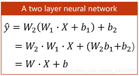
为了提高模型的复杂程度，在每一个线性层的最终输出增加一个非线性变换函数（激活函数）。

3.2 链式求导法则

反向传播示例：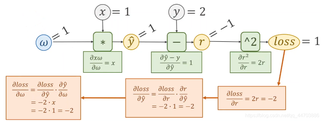

3.3 pytorch实现反向传播

在pytorch中张量包含权重的值和损失对权重的导数

import torch
x_data = [1.0,2.0,3.0]
y_data = [2.0,4.0,6.0]
w = torch.Tensor([1.0])  # 张量
w.requires_grad = True  # 需要计算梯度

# 只要含有张量，定义的函数不再是简单的计算，而是构建计算图
def forward(x):
    return x*w

def loss(x,y):
    y_pred = forward(x)
    return (y_pred-y)**2

# 训练
print('predict(before training)',4,forward(4).item())
for epoch in range(100):
    for x,y in zip(x_data,y_data):
        l = loss(x,y)  # 张量
        l.backward()  # 反向传播，自动存到w，同时计算图释放
        print('\tgrad:',x,y,w.grad.item())
        w.data = w.data - 0.01*w.grad.data  # 权重更新
        w.grad.data.zero_()  # 梯度清零

    print('progress:',epoch,l.item())
print('predict(after training)',4,forward(4).item())