当前位置:网站首页>多种深度模型实现手写字母MNIST的识别(CNN,RNN,DNN,逻辑回归,CRNN,LSTM/Bi-LSTM,GRU/Bi-GRU)
多种深度模型实现手写字母MNIST的识别(CNN,RNN,DNN,逻辑回归,CRNN,LSTM/Bi-LSTM,GRU/Bi-GRU)
2022-08-10 18:23:00 【王延凯的博客】
多种深度模型实现手写字母MNIST的识别(CNN,RNN,DNN,逻辑回归,CRNN,LSTM/Bi-LSTM,GRU/Bi-GRU
1.CNN模型
1.1 代码
import torch
import torch.nn as nn
from torch.autograd import Variable
import torch.utils.data as Data
import torchvision
import matplotlib.pyplot as plt

# Hyper prameters
EPOCH = 1
BATCH_SIZE = 50
LR = 0.001
DOWNLOAD_MNIST = True

train_data = torchvision.datasets.MNIST(
    root='./mnist',
    train=True,
    transform=torchvision.transforms.ToTensor(),  # 将下载的文件转换成pytorch认识的tensor类型,且将图片的数值大小从(0-255)归一化到(0-1)
    download=DOWNLOAD_MNIST
)

# 画一个图片显示出来
# print(train_data.data.size())
# print(train_data.targets.size())
# plt.imshow(train_data.data[0].numpy(),cmap='gray')
# plt.title('%i'%train_data.targets[0])
# plt.show()

train_loader = Data.DataLoader(dataset=train_data, batch_size=BATCH_SIZE, shuffle=True)

test_data = torchvision.datasets.MNIST(
    root='./mnist',
    train=False,
)
with torch.no_grad():
    test_x = Variable(torch.unsqueeze(test_data.data, dim=1)).type(torch.FloatTensor)[
             :2000] / 255  # 只取前两千个数据吧,差不多已经够用了,然后将其归一化。
    test_y = test_data.targets[:2000]

'''开始建立CNN网络'''


class CNN(nn.Module):
    def __init__(self):
        super(CNN, self).__init__()
        '''
        一般来说,卷积网络包括以下内容:
        1.卷积层
        2.神经网络
        3.池化层
        '''
        self.conv1 = nn.Sequential(
            nn.Conv2d(  # --> (1,28,28)
                in_channels=1,  # 传入的图片是几层的,灰色为1层,RGB为三层
                out_channels=16,  # 输出的图片是几层
                kernel_size=5,  # 代表扫描的区域点为5*5
                stride=1,  # 就是每隔多少步跳一下
                padding=2,  # 边框补全,其计算公式=(kernel_size-1)/2=(5-1)/2=2
            ),  # 2d代表二维卷积           --> (16,28,28)
            nn.ReLU(),  # 非线性激活层
            nn.MaxPool2d(kernel_size=2),  # 设定这里的扫描区域为2*2,且取出该2*2中的最大值          --> (16,14,14)
        )

        self.conv2 = nn.Sequential(
            nn.Conv2d(  # --> (16,14,14)
                in_channels=16,  # 这里的输入是上层的输出为16层
                out_channels=32,  # 在这里我们需要将其输出为32层
                kernel_size=5,  # 代表扫描的区域点为5*5
                stride=1,  # 就是每隔多少步跳一下
                padding=2,  # 边框补全,其计算公式=(kernel_size-1)/2=(5-1)/2=
            ),  # --> (32,14,14)
            nn.ReLU(),
            nn.MaxPool2d(kernel_size=2),  # 设定这里的扫描区域为2*2,且取出该2*2中的最大值     --> (32,7,7),这里是三维数据
        )

        self.out = nn.Linear(32 * 7 * 7, 10)  # 注意一下这里的数据是二维的数据

    def forward(self, x):
        x = self.conv1(x)
        x = self.conv2(x)  # (batch,32,7,7)
        # 然后接下来进行一下扩展展平的操作,将三维数据转为二维的数据
        x = x.view(x.size(0), -1)  # (batch ,32 * 7 * 7)
        output = self.out(x)
        return output


cnn = CNN()
# print(cnn)

# 添加优化方法
optimizer = torch.optim.Adam(cnn.parameters(), lr=LR)
# 指定损失函数使用交叉信息熵
loss_fn = nn.CrossEntropyLoss()

'''
开始训练我们的模型哦
'''
step = 0
for epoch in range(EPOCH):
    # 加载训练数据
    for step, data in enumerate(train_loader):
        x, y = data
        # 分别得到训练数据的x和y的取值
        b_x = Variable(x)
        b_y = Variable(y)

        output = cnn(b_x)  # 调用模型预测
        loss = loss_fn(output, b_y)  # 计算损失值
        optimizer.zero_grad()  # 每一次循环之前,将梯度清零
        loss.backward()  # 反向传播
        optimizer.step()  # 梯度下降

        # 每执行50次,输出一下当前epoch、loss、accuracy
        if (step % 50 == 0):
            # 计算一下模型预测正确率
            test_output = cnn(test_x)
            y_pred = torch.max(test_output, 1)[1].data.squeeze()
            accuracy = sum(y_pred == test_y).item() / test_y.size(0)

            print('now epoch :  ', epoch, '   |  loss : %.4f ' % loss.item(), '     |   accuracy :   ', accuracy)

'''
打印十个测试集的结果
'''
test_output = cnn(test_x[:10])
y_pred = torch.max(test_output, 1)[1].data.squeeze()  # 选取最大可能的数值所在的位置
print(y_pred.tolist(), 'predecton Result')
print(test_y[:10].tolist(), 'Real Result')
1.2 运行结果

2.RNN模型
2.1 LSTM/Bi-LSTM
import torch
from torch import nn
import torchvision.datasets as dsets
import torchvision.transforms as transforms
# import matplotlib.pyplot as plt
# torch.manual_seed(1) # reproducible
# Hyper Parameters
EPOCH = 1 # train the training data n times, to save time, we just train 1 epoch
BATCH_SIZE = 64
TIME_STEP = 28 # rnn time step / image height
INPUT_SIZE = 28 # rnn input size / image width
LR = 0.01 # learning rate
DOWNLOAD_MNIST = True # set to True if haven't download the data
# Mnist digital dataset
train_data = dsets.MNIST(
root='./mnist/',
train=True, # this is training data
transform=transforms.ToTensor(), # Converts a PIL.Image or numpy.ndarray to
# torch.FloatTensor of shape (C x H x W) and normalize in the range [0.0, 1.0]
download=DOWNLOAD_MNIST, # download it if you don't have it
)
# plot one example
print(train_data.train_data.size()) # (60000, 28, 28)
print(train_data.train_labels.size()) # (60000)
# plt.imshow(train_data.train_data[0].numpy(), cmap='gray')
# plt.title('%i' % train_data.train_labels[0])
# plt.show()
# Data Loader for easy mini-batch return in training
train_loader = torch.utils.data.DataLoader(dataset=train_data, batch_size=BATCH_SIZE, shuffle=True)
# convert test data into Variable, pick 2000 samples to speed up testing
test_data = dsets.MNIST(root='./mnist/', train=False, transform=transforms.ToTensor())
test_x = test_data.test_data.type(torch.FloatTensor)[:2000]/255. # shape (2000, 28, 28) value in range(0,1)
test_y = test_data.test_labels.numpy()[:2000] # covert to numpy array
class RNN(nn.Module):
def __init__(self):
super(RNN, self).__init__()
self.rnn = nn.LSTM( # if use nn.RNN(), it hardly learns
input_size=INPUT_SIZE,
hidden_size=64, # rnn hidden unit
num_layers=1, # number of rnn layer
batch_first=True, # input & output will has batch size as 1s dimension. e.g. (batch, time_step, input_size)
bidirectional=False, #如果是Bi-LSTM的话,需要将bidirectional设置为True,并将下一行的(64,10)改为(64*2,10)
#如果是LSTM的话,保持此设置即可。
)
self.out = nn.Linear(64, 10)
def forward(self, x):
# x shape (batch, time_step, input_size)
# r_out shape (batch, time_step, output_size)
# h_n shape (n_layers, batch, hidden_size)
# h_c shape (n_layers, batch, hidden_size)
r_out, (h_n, h_c) = self.rnn(x, None) # None represents zero initial hidden state
# print('1111111',x.size())
# choose r_out at the last time step
out = self.out(r_out[:, -1, :])
return out
rnn = RNN()
print(rnn)
optimizer = torch.optim.Adam(rnn.parameters(), lr=LR) # optimize all cnn parameters
loss_func = nn.CrossEntropyLoss() # the target label is not one-hotted
# training and testing
for epoch in range(EPOCH):
for step, (b_x, b_y) in enumerate(train_loader): # gives batch data
# print('000',b_x.size())
b_x = b_x.view(-1, 28, 28) # reshape x to (batch, time_step, input_size)
# print("222",b_x.size())
output = rnn(b_x) # rnn output
loss = loss_func(output, b_y) # cross entropy loss
optimizer.zero_grad() # clear gradients for this training step
loss.backward() # backpropagation, compute gradients
optimizer.step() # apply gradients
if step % 50 == 0:
test_output = rnn(test_x) # (samples, time_step, input_size)
pred_y = torch.max(test_output, 1)[1].data.numpy()
accuracy = float((pred_y == test_y).astype(int).sum()) / float(test_y.size)
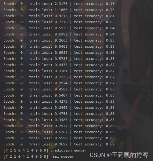
print('Epoch: ', epoch, '| train loss: %.4f' % loss.data.numpy(), '| test accuracy: %.2f' % accuracy)
# print 10 predictions from test data
test_output = rnn(test_x[:10].view(-1, 28, 28))
pred_y = torch.max(test_output, 1)[1].data.numpy()
print(pred_y, 'prediction number')
print(test_y[:10], 'real number')
2.2 运行结果
| LSTM | Bi-LSTM |
|---|---|
 |  |
2.3GRU/Bi-GRU
import time,os
import math
import torch
import torchvision
import torch.nn as nn
import torch.utils.data as Data
import matplotlib.pyplot as plt

class GRUCell(nn.Module):
    """Gated recurrent unit (GRU) cell"""

    def __init__(self, input_size, hidden_size):
        super(GRUCell, self).__init__()
        self.input_size = input_size
        self.hidden_size = hidden_size
        self.weight_ih = nn.Parameter(torch.Tensor(input_size, hidden_size * 3))
        self.weight_hh = nn.Parameter(torch.Tensor(hidden_size, hidden_size * 3))
        self.bias_ih = nn.Parameter(torch.Tensor(hidden_size * 3))
        self.bias_hh = nn.Parameter(torch.Tensor(hidden_size * 3))
        self.init_parameters()

    def init_parameters(self):
        stdv = 1.0 / math.sqrt(self.hidden_size)
        for param in self.parameters():
            nn.init.uniform_(param, -stdv, stdv)

    def forward(self, x, h_t_minus_1):
        idx = self.hidden_size * 2
        gates_ih = torch.mm(x, self.weight_ih) + self.bias_ih
        gates_hh = torch.mm(h_t_minus_1, self.weight_hh[:, :idx]) + self.bias_hh[:idx]
        resetgate_i, updategate_i, output_i = gates_ih.chunk(3, dim=1)
        resetgate_h, updategate_h = gates_hh.chunk(2, dim=1)
        r = torch.sigmoid(resetgate_i + resetgate_h)
        z = torch.sigmoid(updategate_i + updategate_h)
        h_tilde = torch.tanh(output_i + (torch.mm((r * h_t_minus_1), self.weight_hh[:, idx:]) + self.bias_hh[idx:]))
        h = (1 - z) * h_t_minus_1 + z * h_tilde
        return h


class GRU(nn.Module):
    """Multi-layer gated recurrent unit (GRU)"""

    def __init__(self, input_size, hidden_size, num_layers=1, batch_first=False):
        super(GRU, self).__init__()
        self.hidden_size = hidden_size
        self.num_layers = num_layers
        self.batch_first = batch_first
        layers = [GRUCell(input_size, hidden_size)]
        for i in range(num_layers - 1):
            layers += [GRUCell(hidden_size, hidden_size)]
        self.net = nn.Sequential(*layers)

    def forward(self, x, init_state=None):
        # Input and output size: (seq_length, batch_size, input_size)
        # State size: (num_layers, batch_size, hidden_size)
        if self.batch_first:
            x = x.transpose(0, 1)

        self.h = torch.zeros(x.size(0), self.num_layers, x.size(1), self.hidden_size).to(x.device)
        if init_state is not None:
            self.h[0, :] = init_state

        inputs = x
        for i, cell in enumerate(self.net):  # Layers
            h_t = self.h[0, i].clone()
            for t in range(x.size(0)):  # Sequences
                h_t = cell(inputs[t], h_t)
                self.h[t, i] = h_t
            inputs = self.h[:, i].clone()

        if self.batch_first:
            return self.h[:, -1].transpose(0, 1), self.h[-1]

        return self.h[:, -1], self.h[-1]

        # if init_state is not None:
        #     h_0 = init_state
        # else:
        #     h_0 = torch.zeros(self.num_layers, x.size(1), self.hidden_size).to(x.device)
        #
        # inputs, outputs, h = x, [], []
        # for i, cell in enumerate(self.net):  # Layers
        #     h_t = h_0[i]
        #     for t in range(x.size(0)):  # Sequences
        #         h_t = cell(inputs[t], h_t)
        #         outputs += [h_t]
        #     inputs, outputs = outputs, []
        #     h += [h_t]
        #
        # if self.batch_first:
        #     return torch.stack(inputs).transpose(0, 1), torch.stack(h)
        #
        # return torch.stack(inputs), torch.stack(h)


class GRUModel(nn.Module):
    def __init__(self, input_size, hidden_size, num_layers, output_size):
        super(GRUModel, self).__init__()
        self.hidden_size = hidden_size
        self.num_layers = num_layers
        self.gru = GRU(input_size, hidden_size, num_layers, batch_first=True)
        self.fc = nn.Linear(hidden_size, output_size)

    def forward(self, x):
        out, _ = self.gru(x, None)
        out = self.fc(out[:, -1, :])
        return out

'''
超参数设置
'''

learning_rate = 0.001
num_epochs = 1
BATCH_SIZE = 50
print_step = 200

num_layers = 3
input_size = 28
time_step = 28
hidden_size = 128
output_size = 10
DOWNLOAD_MNIST = True


# Mnist digits dataset
if not(os.path.exists('./mnist/')) or not os.listdir('./mnist/'):
    # not mnist dir or mnist is empyt dir
    DOWNLOAD_MNIST = True

train_data = torchvision.datasets.MNIST(
    root='./mnist/',
    train=True,                                     # this is training data
    transform=torchvision.transforms.ToTensor(),    # Converts a PIL.Image or numpy.ndarray to
                                                    # torch.FloatTensor of shape (C x H x W) and normalize in the range [0.0, 1.0]
    download=DOWNLOAD_MNIST,
)

test_data = torchvision.datasets.MNIST(
    root='./mnist/',
    train=False,                                     # this is training data
    transform=torchvision.transforms.ToTensor(),    # Converts a PIL.Image or numpy.ndarray to
                                                    # torch.FloatTensor of shape (C x H x W) and normalize in the range [0.0, 1.0]
    download=DOWNLOAD_MNIST,
)

# plot one example
print(train_data.train_data.size())                 # (60000, 28, 28)
print(train_data.train_labels.size())               # (60000)
# plt.imshow(train_data.train_data[0].numpy(), cmap='gray')
# plt.title('%i' % train_data.train_labels[0])
# plt.show()

# Data Loader for easy mini-batch return in training, the image batch shape will be (50, 1, 28, 28)
train_loader = Data.DataLoader(dataset=train_data, batch_size=BATCH_SIZE, shuffle=True)

# pick 2000 samples to speed up testing
# test_data = torchvision.datasets.MNIST(root='./mnist/', train=False)
test_loader = Data.DataLoader(dataset=test_data, batch_size=BATCH_SIZE, shuffle=True)

# for data,labels in test_loader:
#     print(data,labels)

test_x = torch.unsqueeze(test_data.test_data, dim=1).type(torch.FloatTensor)[:2000]/255.   # shape from (2000, 28, 28) to (2000, 1, 28, 28), value in range(0,1)
test_y = test_data.test_labels[:2000]


device = torch.device('cuda' if torch.cuda.is_available() else 'cpu')


model = GRUModel(input_size, hidden_size, num_layers, output_size).to(device)

criterion = nn.CrossEntropyLoss()
optimizer = torch.optim.Adam(model.parameters(), lr=learning_rate)

start = time.time()

steps = len(train_loader)
test_total = len(test_loader.dataset)

print('Train on {} samples, test on {} samples'.format(len(train_loader.dataset), test_total))

for epoch in range(num_epochs):
    print('Epoch {}/{}'.format(epoch + 1, num_epochs))

    running_loss = 0.0
    corrects = 0
    total = 0

    for i, (inputs, labels) in enumerate(train_loader):
        inputs = inputs.view(-1, time_step, input_size).to(device)
        labels = labels.to(device, non_blocking=True)

        # Clear the gradients
        optimizer.zero_grad()

        # Forward pass
        outputs = model(inputs)

        loss = criterion(outputs, labels)

        # Backward and optimize
        loss.backward()
        optimizer.step()

        # Statistics
        running_loss += loss.item() * inputs.size(0)
        _, preds = torch.max(outputs, 1)
        corrects += torch.sum(preds == labels).item()
        total += inputs.size(0)

        if (i + 1) % print_step == 0 or (i + 1) == steps:
            # Test phase
            test_running_loss = 0.0
            test_corrects = 0

            for inputs, labels in test_loader:
                inputs = inputs.view(-1, time_step, input_size).to(device)
                labels = labels.to(device)

                # Prevent tracking history
                with torch.no_grad():
                    outputs = model(inputs)

                    loss = criterion(outputs, labels)

                    test_running_loss += loss.item() * inputs.size(0)
                    _, preds = torch.max(outputs, 1)
                    test_corrects += torch.sum(preds == labels).item()

            train_acc = corrects / total
            train_loss = running_loss / total
            test_acc = test_corrects / test_total
            test_loss = test_running_loss / test_total

            print('step: {}/{} - loss: {:.4f} - acc: {:.3f} - test_loss: {:.4f} - test_acc: {:.3f}'.format(
                i + 1, steps, train_loss, train_acc, test_loss, test_acc))

elapsed_time = time.time() - start
print('Training complete in {:.0f}m {:.0f}s'.format(elapsed_time // 60, elapsed_time % 60))

inputs = inputs.cpu().numpy()
preds = preds.cpu().numpy()
labels = labels.cpu().numpy()
n_rows, n_cols = (2, 8)
plt.figure(figsize=(n_cols, n_rows))
for i in range(n_rows * n_cols):
    plt.subplot(n_rows, n_cols, i + 1)
    plt.axis('off')
    plt.title(preds[i])
    plt.imshow(inputs[i], cmap='gray')
plt.tight_layout()
plt.show()
3.DNN模型
3.1 代码
import os
import torch
import torchvision
import torch.nn as nn
import torch.nn.functional as F
import torch.utils.data as Data


class mnist_DNN_model(nn.Module):
    def __init__(self):
        super(mnist_DNN_model, self).__init__()
        self.model_path = 'torch_model'
        self.model_name = 'mnist_DNN_model'

        self.dropout_p = 0.5

        self.sequential_1 = nn.Sequential(
            nn.Linear(28*28, 512),
            nn.BatchNorm1d(512),
            nn.ReLU(),
            nn.Dropout(self.dropout_p)
        )

        self.fc_2 = nn.Linear(512, 256)
        self.bn_2 = nn.BatchNorm1d(256)
        self.d_3 = nn.Dropout(self.dropout_p)

        self.fc_3 = nn.Linear(256, 128)
        self.bn_3 = nn.BatchNorm1d(128)
        self.d_3 = nn.Dropout(self.dropout_p)

        self.fc_oupt = nn.Linear(128, 10)

    def forward(self, x):
        re_x = x.view((-1, 28*28))

        fc_1 = self.sequential_1(re_x)

        fc_2 = self.fc_2(fc_1)
        bn_2 = F.relu(self.bn_2(fc_2))
        d_2 = self.d_3(bn_2)

        fc_3 = self.fc_3(d_2)
        bn_3 = F.elu(self.bn_3(fc_3))
        d_3 = self.d_3(bn_3)

        fc_oupt = self.fc_oupt(d_3)

        return F.log_softmax(fc_oupt)

# Hyper Parameters
EPOCH = 1               # train the training data n times, to save time, we just train 1 epoch
BATCH_SIZE = 50
LR = 0.001              # learning rate
DOWNLOAD_MNIST = False


# Mnist digits dataset
if not(os.path.exists('./mnist/')) or not os.listdir('./mnist/'):
    # not mnist dir or mnist is empyt dir
    DOWNLOAD_MNIST = True

train_data = torchvision.datasets.MNIST(
    root='./mnist/',
    train=True,                                     # this is training data
    transform=torchvision.transforms.ToTensor(),    # Converts a PIL.Image or numpy.ndarray to
                                                    # torch.FloatTensor of shape (C x H x W) and normalize in the range [0.0, 1.0]
    download=DOWNLOAD_MNIST,
)

# plot one example
print(train_data.train_data.size())                 # (60000, 28, 28)
print(train_data.train_labels.size())               # (60000)
# plt.imshow(train_data.train_data[0].numpy(), cmap='gray')
# plt.title('%i' % train_data.train_labels[0])
# plt.show()

# Data Loader for easy mini-batch return in training, the image batch shape will be (50, 1, 28, 28)
train_loader = Data.DataLoader(dataset=train_data, batch_size=BATCH_SIZE, shuffle=True)

# pick 2000 samples to speed up testing
test_data = torchvision.datasets.MNIST(root='./mnist/', train=False)
test_x = torch.unsqueeze(test_data.test_data, dim=1).type(torch.FloatTensor)[:2000]/255.   # shape from (2000, 28, 28) to (2000, 1, 28, 28), value in range(0,1)
test_y = test_data.test_labels[:2000]


device = torch.device('cuda' if torch.cuda.is_available() else 'cpu')
model = mnist_DNN_model().to(device)
print(model)

optimizer = torch.optim.Adam(model.parameters(), lr=LR)   # optimize all logistic parameters
loss_func = nn.CrossEntropyLoss()                       # the target label is not one-hotted


for epoch in range(EPOCH):
    for step, (b_x, b_y) in enumerate(train_loader):   # gives batch data, normalize x when iterate train_loader
        # print(b_x.size())
        # b_x = b_x.view(-1, 28*28)
        # print(b_x.size())

        output = model(b_x)               # logistic output
        loss = loss_func(output, b_y)   # cross entropy loss
        optimizer.zero_grad()           # clear gradients for this training step
        loss.backward()                 # backpropagation, compute gradients
        optimizer.step()                # apply gradients

        if step % 50 == 0:

            test_output = model(test_x)
            pred_y = torch.max(test_output, 1)[1].data.numpy()
            accuracy = float((pred_y == test_y.data.numpy()).astype(int).sum()) / float(test_y.size(0))
            print('Epoch: ', epoch, '| train loss: %.4f' % loss.data.numpy(), '| test accuracy: %.2f' % accuracy)
            # if HAS_SK:
            #     # Visualization of trained flatten layer (T-SNE)
            #     tsne = TSNE(perplexity=30, n_components=2, init='pca', n_iter=5000)
            #     plot_only = 500
            #     low_dim_embs = tsne.fit_transform(last_layer.data.numpy()[:plot_only, :])
            #     labels = test_y.numpy()[:plot_only]
            #     plot_with_labels(low_dim_embs, labels)
# plt.ioff()

# print 10 predictions from test data
test_output = model(test_x[:10])
pred_y = torch.max(test_output, 1)[1].data.numpy()
print(pred_y, 'prediction number')
print(test_y[:10].numpy(), 'real number')
3.2 运行结果

4.逻辑回归模型
4.1 代码
import os

import torch
import torch.nn as nn
import torch.utils.data as Data
import torchvision
# import matplotlib.pyplot as plt

# torch.manual_seed(1)    # reproducible

# Hyper Parameters
EPOCH = 1               # train the training data n times, to save time, we just train 1 epoch
BATCH_SIZE = 50
LR = 0.001              # learning rate
DOWNLOAD_MNIST = False


# Mnist digits dataset
if not(os.path.exists('./mnist/')) or not os.listdir('./mnist/'):
    # not mnist dir or mnist is empyt dir
    DOWNLOAD_MNIST = True

train_data = torchvision.datasets.MNIST(
    root='./mnist/',
    train=True,                                     # this is training data
    transform=torchvision.transforms.ToTensor(),    # Converts a PIL.Image or numpy.ndarray to
                                                    # torch.FloatTensor of shape (C x H x W) and normalize in the range [0.0, 1.0]
    download=DOWNLOAD_MNIST,
)

# plot one example
print(train_data.train_data.size())                 # (60000, 28, 28)
print(train_data.train_labels.size())               # (60000)
# plt.imshow(train_data.train_data[0].numpy(), cmap='gray')
# plt.title('%i' % train_data.train_labels[0])
# plt.show()

# Data Loader for easy mini-batch return in training, the image batch shape will be (50, 1, 28, 28)
train_loader = Data.DataLoader(dataset=train_data, batch_size=BATCH_SIZE, shuffle=True)

# pick 2000 samples to speed up testing
test_data = torchvision.datasets.MNIST(root='./mnist/', train=False)
test_x = torch.unsqueeze(test_data.test_data, dim=1).type(torch.FloatTensor)[:2000]/255.   # shape from (2000, 28, 28) to (2000, 1, 28, 28), value in range(0,1)
test_y = test_data.test_labels[:2000]


class logisticRg(nn.Module):
    def __init__(self):
        super(logisticRg, self).__init__()
        self.lr = nn.Sequential(
            nn.Linear(28*28,10)
        )

    def forward(self, x):
        output = self.lr(x)
        return output, x    # return x for visualization


lor = logisticRg()
print(lor)  # net architecture

optimizer = torch.optim.Adam(lor.parameters(), lr=LR)   # optimize all logistic parameters
loss_func = nn.CrossEntropyLoss()                       # the target label is not one-hotted

# following function (plot_with_labels) is for visualization, can be ignored if not interested
# from matplotlib import cm
# try: from sklearn.manifold import TSNE; HAS_SK = True
# except: HAS_SK = False; print('Please install sklearn for layer visualization')
# def plot_with_labels(lowDWeights, labels):
#     plt.cla()
#     X, Y = lowDWeights[:, 0], lowDWeights[:, 1]
#     for x, y, s in zip(X, Y, labels):
#         c = cm.rainbow(int(255 * s / 9)); plt.text(x, y, s, backgroundcolor=c, fontsize=9)
#     plt.xlim(X.min(), X.max()); plt.ylim(Y.min(), Y.max()); plt.title('Visualize last layer'); plt.show(); plt.pause(0.01)

# plt.ion()
# training and testing
for epoch in range(EPOCH):
    for step, (b_x, b_y) in enumerate(train_loader):   # gives batch data, normalize x when iterate train_loader
        # print(b_x.size())
        b_x = b_x.view(-1, 28*28)
        # print(b_x.size())

        output = lor(b_x)[0]               # logistic output
        loss = loss_func(output, b_y)   # cross entropy loss
        optimizer.zero_grad()           # clear gradients for this training step
        loss.backward()                 # backpropagation, compute gradients
        optimizer.step()                # apply gradients

        if step % 50 == 0:

            test_output, last_layer = lor(test_x.view(-1,28*28))
            pred_y = torch.max(test_output, 1)[1].data.numpy()
            accuracy = float((pred_y == test_y.data.numpy()).astype(int).sum()) / float(test_y.size(0))
            print('Epoch: ', epoch, '| train loss: %.4f' % loss.data.numpy(), '| test accuracy: %.2f' % accuracy)
            # if HAS_SK:
            #     # Visualization of trained flatten layer (T-SNE)
            #     tsne = TSNE(perplexity=30, n_components=2, init='pca', n_iter=5000)
            #     plot_only = 500
            #     low_dim_embs = tsne.fit_transform(last_layer.data.numpy()[:plot_only, :])
            #     labels = test_y.numpy()[:plot_only]
            #     plot_with_labels(low_dim_embs, labels)
# plt.ioff()

# print 10 predictions from test data
test_output, _ = lor(test_x[:10].view(-1,28*28))
pred_y = torch.max(test_output, 1)[1].data.numpy()
print(pred_y, 'prediction number')
print(test_y[:10].numpy(), 'real number')
4.2 运行结果
5.CRNN模型(CNN-LSTM/CNN-Bi-LSTM)
5.1代码
import torch
import torch.nn as nn
from torch.autograd import Variable
import torch.utils.data as Data
import torchvision
import matplotlib.pyplot as plt

# Hyper prameters
EPOCH = 1
BATCH_SIZE = 50
LR = 0.0001
DOWNLOAD_MNIST = True

train_data = torchvision.datasets.MNIST(
    root='./mnist',
    train=True,
    transform=torchvision.transforms.ToTensor(),  # 将下载的文件转换成pytorch认识的tensor类型,且将图片的数值大小从(0-255)归一化到(0-1)
    download=DOWNLOAD_MNIST
)

# 画一个图片显示出来
# print(train_data.data.size())
# print(train_data.targets.size())
# plt.imshow(train_data.data[0].numpy(),cmap='gray')
# plt.title('%i'%train_data.targets[0])
# plt.show()

train_loader = Data.DataLoader(dataset=train_data, batch_size=BATCH_SIZE, shuffle=True)

test_data = torchvision.datasets.MNIST(
    root='./mnist',
    train=False,
)
with torch.no_grad():
    test_x = Variable(torch.unsqueeze(test_data.data, dim=1)).type(torch.FloatTensor)[
             :2000] / 255  # 只取前两千个数据吧,差不多已经够用了,然后将其归一化。
    test_y = test_data.targets[:2000]

'''开始建立CNN网络'''


class CRNN(nn.Module):
    def __init__(self):
        super(CRNN, self).__init__()
        '''
        一般来说,卷积网络包括以下内容:
        1.卷积层
        2.神经网络
        3.池化层
        '''
        self.conv1 = nn.Sequential(
            nn.Conv2d(  # --> (1,28,28)
                in_channels=1,  # 传入的图片是几层的,灰色为1层,RGB为三层
                out_channels=16,  # 输出的图片是几层
                kernel_size=5,  # 代表扫描的区域点为5*5
                stride=1,  # 就是每隔多少步跳一下
                padding=2,  # 边框补全,其计算公式=(kernel_size-1)/2=(5-1)/2=2
            ),  # 2d代表二维卷积           --> (16,28,28)
            nn.ReLU(),  # 非线性激活层
            nn.MaxPool2d(kernel_size=2),  # 设定这里的扫描区域为2*2,且取出该2*2中的最大值          --> (16,14,14)
        )

        self.conv2 = nn.Sequential(
            nn.Conv2d(  # --> (16,14,14)
                in_channels=16,  # 这里的输入是上层的输出为16层
                out_channels=49,  # 在这里我们需要将其输出为32层
                kernel_size=5,  # 代表扫描的区域点为5*5
                stride=1,  # 就是每隔多少步跳一下
                padding=2,  # 边框补全,其计算公式=(kernel_size-1)/2=(5-1)/2=
            ),  # --> (32,14,14)
            nn.ReLU(),
            nn.MaxPool2d(kernel_size=2),  # 设定这里的扫描区域为2*2,且取出该2*2中的最大值     --> (32,7,7),这里是三维数据
        )

        self.lstm=nn.LSTM(input_size=49,hidden_size=100,num_layers=1,bidirectional=False)  #输入为32*7*7,隐藏层为100,双向

        self.out = nn.Linear(100, 10)  # 注意一下这里的数据是二维的数据

    def forward(self, x):
        x = self.conv1(x)
        x = self.conv2(x)  # (batch,32,7,7)
        # 然后接下来进行一下扩展展平的操作,将三维数据转为二维的数据
        # print("000",x.size())
        # x = x.view(x.size(0), -1)  # (batch ,32 * 7 * 7)
        x=x.reshape(x.size(0),7*7,7*7)
        # print('111',x.size())
        # print('222',y.size())

        r_out, (h_n, h_c)=self.lstm(x)  #这里需要输入三维数据,应该为(batch,*,*)
        # print("333",r_out.size())
        output = self.out(r_out[:, -1, :])
        return output


crnn = CRNN()
# print(cnn)

# 添加优化方法
optimizer = torch.optim.Adam(crnn.parameters(), lr=LR)
# 指定损失函数使用交叉信息熵
loss_fn = nn.CrossEntropyLoss()

'''
开始训练我们的模型哦
'''
step = 0
for epoch in range(EPOCH):
    # 加载训练数据
    for step, data in enumerate(train_loader):
        x, y = data
        # 分别得到训练数据的x和y的取值
        b_x = Variable(x)
        b_y = Variable(y)

        output = crnn(b_x)  # 调用模型预测
        loss = loss_fn(output, b_y)  # 计算损失值
        optimizer.zero_grad()  # 每一次循环之前,将梯度清零
        loss.backward()  # 反向传播
        optimizer.step()  # 梯度下降

        # 每执行50次,输出一下当前epoch、loss、accuracy
        if (step % 50 == 0):
            # 计算一下模型预测正确率
            test_output = crnn(test_x)
            y_pred = torch.max(test_output, 1)[1].data.squeeze()
            accuracy = sum(y_pred == test_y).item() / test_y.size(0)

            print('now epoch :  ', epoch, '   |  loss : %.4f ' % loss.item(), '     |   accuracy :   ', accuracy)

'''
打印十个测试集的结果
'''
test_output = crnn(test_x[:10])
y_pred = torch.max(test_output, 1)[1].data.squeeze()  # 选取最大可能的数值所在的位置
print(y_pred.tolist(), 'predecton Result')
print(test_y[:10].tolist(), 'Real Result')
5.2 运行结果

边栏推荐
猜你喜欢
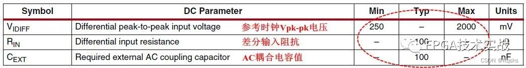
Xilinx FPGA收发器参考时钟设计应用

Toronto Research Chemicals BTK抑制剂丨ACP-5197
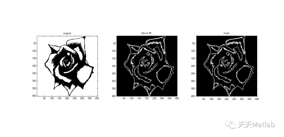
【图像分割】基于元胞自动机实现图像分割附matlab代码

Major upgrade of MSE Governance Center - Traffic Governance, Database Governance, Same AZ Priority
三星Galaxy Watch5产品图片流出 非Pro表款亦有蓝宝石加持

Go 语言快速入门指南:第四篇 与数据为舞之数组

阿里云贾朝辉:云 XR 平台支持彼真科技呈现国风科幻虚拟演唱会

宝塔部署flask项目
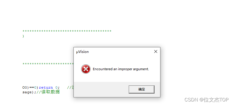
Keil5退出仿真调试卡死的解决办法

运维如何学习、自我提升价值?

随机推荐
消息队列初见:一起聊聊引入系统mq 之后的问题
欧洲核子研究中心首次在量子机器学习研究中取得实效
FPGA工程师面试试题集锦81~90
websocket校验token:使用threadlocal存放和获取当前登录用户
智能出价策略如何影响广告效果?
flex&bison系列第一章:flex Hello World
接口测试进阶接口脚本使用—apipost(预/后执行脚本)
破解校园数字安全难点,联想推出智慧教育安全体系
装饰者模式
FlexSim仿真软件入门笔记:基本操作、快捷键
从企业的视角来看,数据中台到底意味着什么?
三星Galaxy Watch5产品图片流出 非Pro表款亦有蓝宝石加持
幕维三维动画——港珠澳大桥沉管安装三维动画实况
【深度学习21天学习挑战赛】4、初尝循环神经网络(RNN)——股票预测
多线程与高并发(五)—— 源码解析 ReentrantLock
开源一夏 | mysql5.7 安装部署 -二进制安装
漫谈测试成长之探索——测试文档
一小时搞定 简单VBA编程 Excel宏编程快速扫盲
flex使用align-content无效
MySQL安装步骤