当前位置:网站首页>深度学习100例 —— 卷积神经网络(CNN)识别眼睛状态
深度学习100例 —— 卷积神经网络(CNN)识别眼睛状态
2022-08-11 08:52:00 【Ding Jiaxiong】
活动地址:CSDN21天学习挑战赛
深度学习100例——卷积神经网络(CNN)识别眼睛状态
- 本文为365天深度学习训练营 中的学习记录博客
- 参考文章地址: 深度学习100例-卷积神经网络(CNN)识别眼睛状态 | 第17天
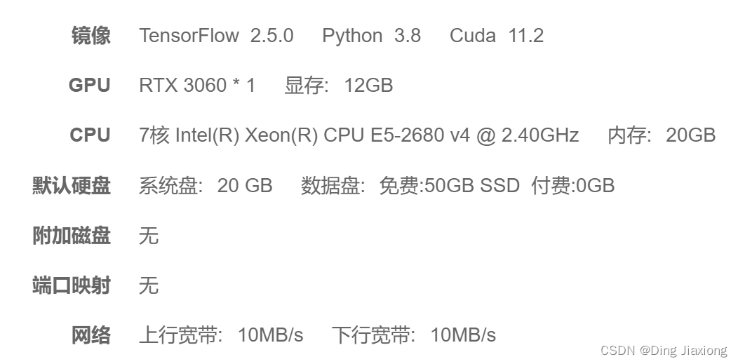
我的环境
1. 前期准备工作
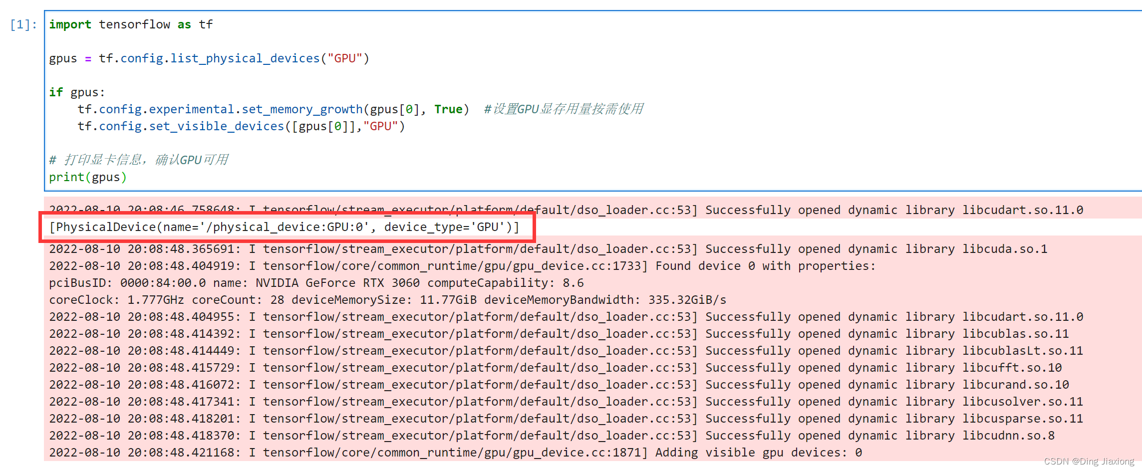
1.1 设置GPU
import tensorflow as tf

gpus = tf.config.list_physical_devices("GPU")

if gpus:
    tf.config.experimental.set_memory_growth(gpus[0], True)  #设置GPU显存用量按需使用
    tf.config.set_visible_devices([gpus[0]],"GPU")

# 打印显卡信息,确认GPU可用
print(gpus)
1.2 导入数据
import matplotlib.pyplot as plt
# 支持中文
plt.rcParams['font.sans-serif'] = ['SimHei']  # 用来正常显示中文标签
plt.rcParams['axes.unicode_minus'] = False  # 用来正常显示负号

import os,PIL

# 设置随机种子尽可能使结果可以重现
import numpy as np
np.random.seed(1)

# 设置随机种子尽可能使结果可以重现
import tensorflow as tf
tf.random.set_seed(1)

import pathlib
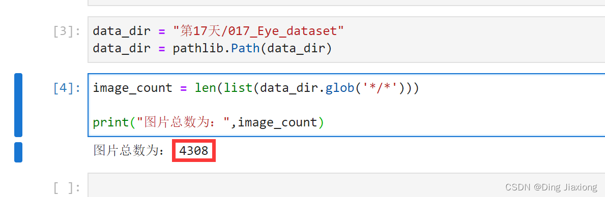
data_dir = "第17天/017_Eye_dataset"
data_dir = pathlib.Path(data_dir)
1.3 查看数据
image_count = len(list(data_dir.glob('*/*')))

print("图片总数为:",image_count)
2. 数据预处理
2.1 加载数据
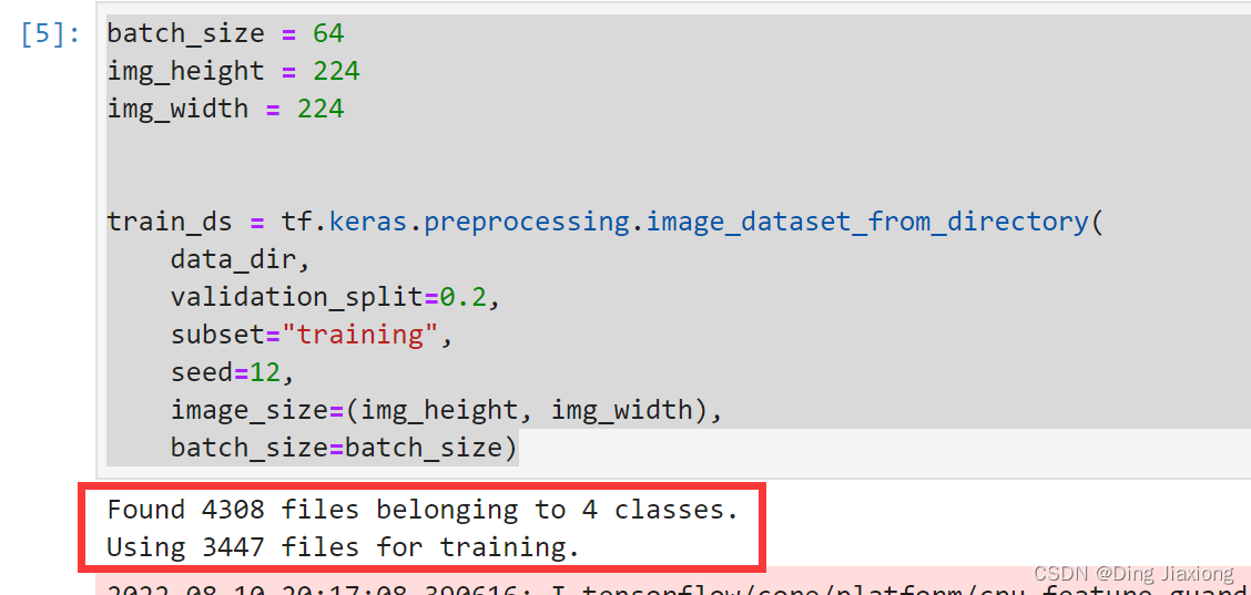
batch_size = 64
img_height = 224
img_width = 224


train_ds = tf.keras.preprocessing.image_dataset_from_directory(
    data_dir,
    validation_split=0.2,
    subset="training",
    seed=12,
    image_size=(img_height, img_width),
    batch_size=batch_size)
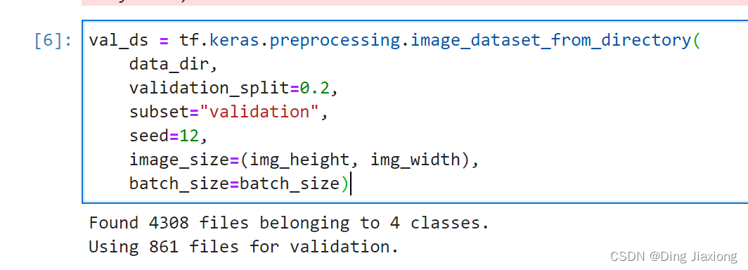
val_ds = tf.keras.preprocessing.image_dataset_from_directory(
    data_dir,
    validation_split=0.2,
    subset="validation",
    seed=12,
    image_size=(img_height, img_width),
    batch_size=batch_size)
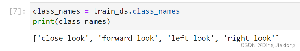
通过class_names输出数据集的标签。标签将按字母顺序对应于目录名称。
class_names = train_ds.class_names
print(class_names)
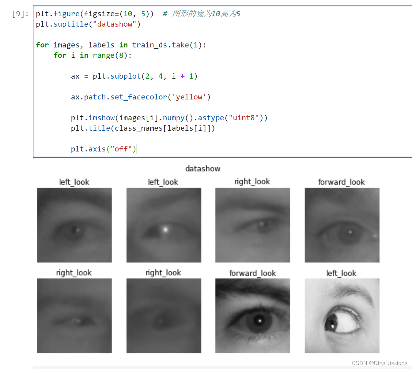
2.2 可视化数据
plt.figure(figsize=(10, 5))  # 图形的宽为10高为5
plt.suptitle("datashow")

for images, labels in train_ds.take(1):
    for i in range(8):

        ax = plt.subplot(2, 4, i + 1)

        ax.patch.set_facecolor('yellow')

        plt.imshow(images[i].numpy().astype("uint8"))
        plt.title(class_names[labels[i]])

        plt.axis("off")
2.3 再次检查数据
for image_batch, labels_batch in train_ds:
    print(image_batch.shape)
    print(labels_batch.shape)
    break
- Image_batch是形状的张量(8,224,224,3)。这是一批形状240x240x3的8张图片(最后一维指的是彩色通道RGB)。
- Label_batch是形状(8,)的张量,这些标签对应8张图片
2.4 配置数据集
shuffle():打乱数据。
prefetch():预取数据,加速运行。
cache():将数据集缓存到内存当中,加速运行。
AUTOTUNE = tf.data.AUTOTUNE

train_ds = train_ds.cache().shuffle(1000).prefetch(buffer_size=AUTOTUNE)
val_ds   = val_ds.cache().prefetch(buffer_size=AUTOTUNE)
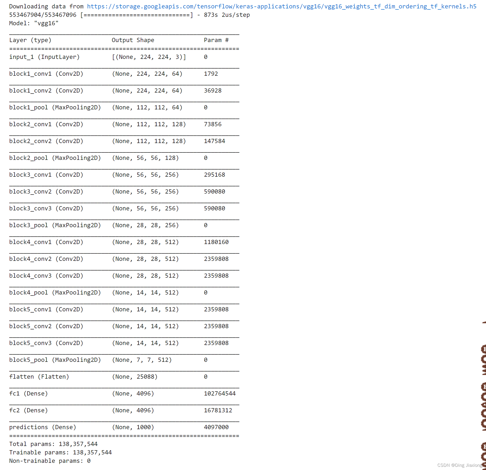
3. 调用官方模型
model = tf.keras.applications.VGG16()
# 打印模型信息
model.summary()
4. 设置动态学习率
- 学习率大
- 优点:1、加快学习速率。2、有助于跳出局部最优值。
- 缺点:1、导致模型训练不收敛。2、单单使用大学习率容易导致模型不精确。
- 学习率小
- 优点:1、有助于模型收敛、模型细化。2、提高模型精度。
- 缺点:1、很难跳出局部最优值。2、收敛缓慢。
注意:这里设置的动态学习率为:指数衰减型(ExponentiaIDecay)。假设1个epoch有100个batch(相当于100step),20个epoch过后,step==2000,即step会随着epoch累加。计算公式如下:
learning _rate = initial_learning_rate *decay_rate ^(step / decay_steps)
# 设置初始学习率
initial_learning_rate = 1e-4

lr_schedule = tf.keras.optimizers.schedules.ExponentialDecay(
        initial_learning_rate,
        decay_steps=20,      # 敲黑板!!!这里是指 steps,不是指epochs
        decay_rate=0.96,     # lr经过一次衰减就会变成 decay_rate*lr
        staircase=True)

# 将指数衰减学习率送入优化器
optimizer = tf.keras.optimizers.Adam(learning_rate=lr_schedule)
5. 编译
- 损失函数(loss):用于衡量模型在训练期间的准确率。
- 优化器(optimizer) :决定模型如何根据其看到的数据和自身的损失函数进行更新。
- 评价函数(metrics) :用于监控训练和测试步骤。以下示例使用了准确率。即被正确分类的图像的比率。
model.compile(optimizer=optimizer,loss ='sparse_categorical_crossentropy',metrics = ['accuracy'])
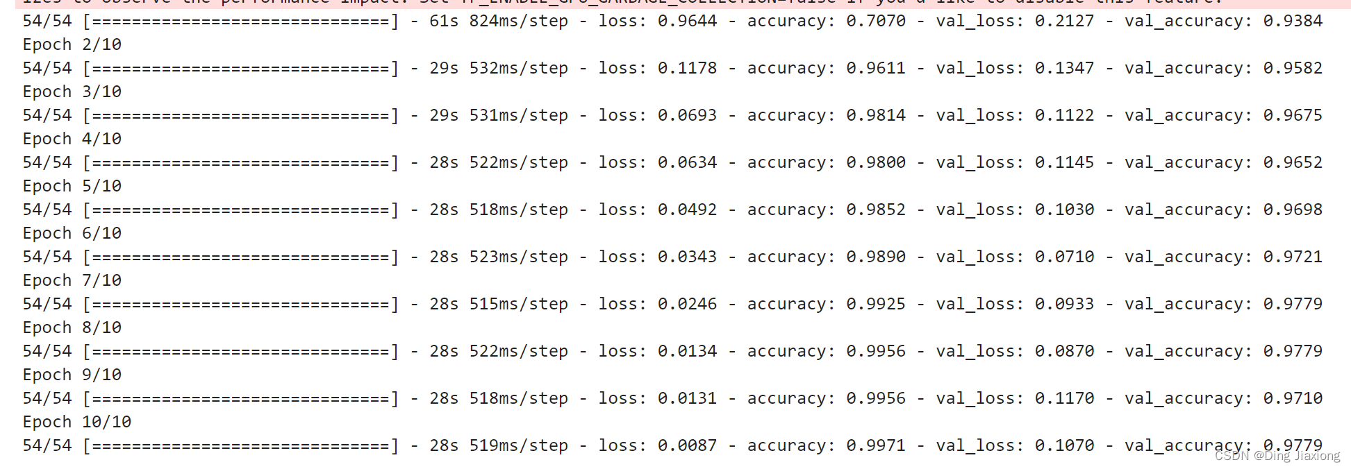
6. 训练模型
epochs = 10

history = model.fit(train_ds,validation_data=val_ds,epochs=epochs)
7. 模型评估
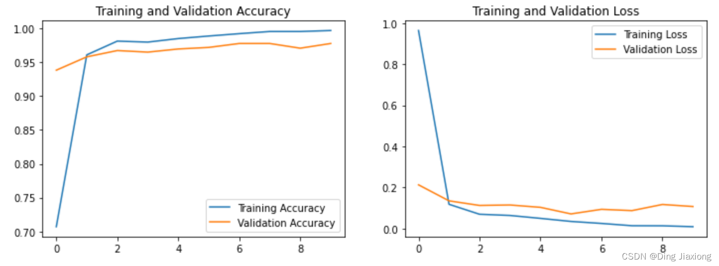
7.1 Accuracy图与Loss图
acc = history.history['accuracy']
val_acc = history.history['val_accuracy']

loss = history.history['loss']
val_loss = history.history['val_loss']

epochs_range = range(epochs)

plt.figure(figsize=(12, 4))
plt.subplot(1, 2, 1)

plt.plot(epochs_range, acc, label='Training Accuracy')
plt.plot(epochs_range, val_acc, label='Validation Accuracy')
plt.legend(loc='lower right')
plt.title('Training and Validation Accuracy')

plt.subplot(1, 2, 2)
plt.plot(epochs_range, loss, label='Training Loss')
plt.plot(epochs_range, val_loss, label='Validation Loss')
plt.legend(loc='upper right')
plt.title('Training and Validation Loss')
plt.show()
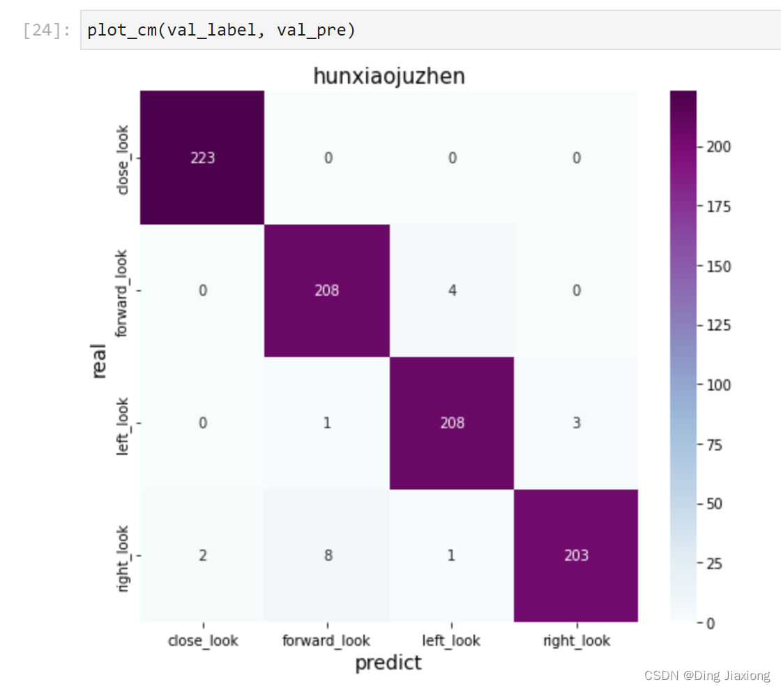
7.2 混淆矩阵
Seaborn是一个画图库,它基于Matplotlib核心库进行了更高阶的API封装,可以让你轻松地画出更漂亮的图形。Seaborn 的漂亮主要体现在配色更加舒服、以及图形元素的样式更加细腻。
from sklearn.metrics import confusion_matrix
import seaborn as sns
import pandas as pd

# 定义一个绘制混淆矩阵图的函数
def plot_cm(labels, predictions):

    # 生成混淆矩阵
    conf_numpy = confusion_matrix(labels, predictions)
    # 将矩阵转化为 DataFrame
    conf_df = pd.DataFrame(conf_numpy, index=class_names ,columns=class_names)

    plt.figure(figsize=(8,7))

    sns.heatmap(conf_df, annot=True, fmt="d", cmap="BuPu")

    plt.title('hunxiaojuzhen',fontsize=15)
    plt.ylabel('real',fontsize=14)
    plt.xlabel('predict',fontsize=14)
val_pre   = []
val_label = []

for images, labels in val_ds:#这里可以取部分验证数据(.take(1))生成混淆矩阵
    for image, label in zip(images, labels):
        # 需要给图片增加一个维度
        img_array = tf.expand_dims(image, 0)
        # 使用模型预测图片中的人物
        prediction = model.predict(img_array)

        val_pre.append(class_names[np.argmax(prediction)])
        val_label.append(class_names[label])
plot_cm(val_label, val_pre)
8. 保存和加载模型
# 保存模型
model.save('model/17_model.h5')
# 加载模型
new_model = tf.keras.models.load_model('model/17_model.h5')
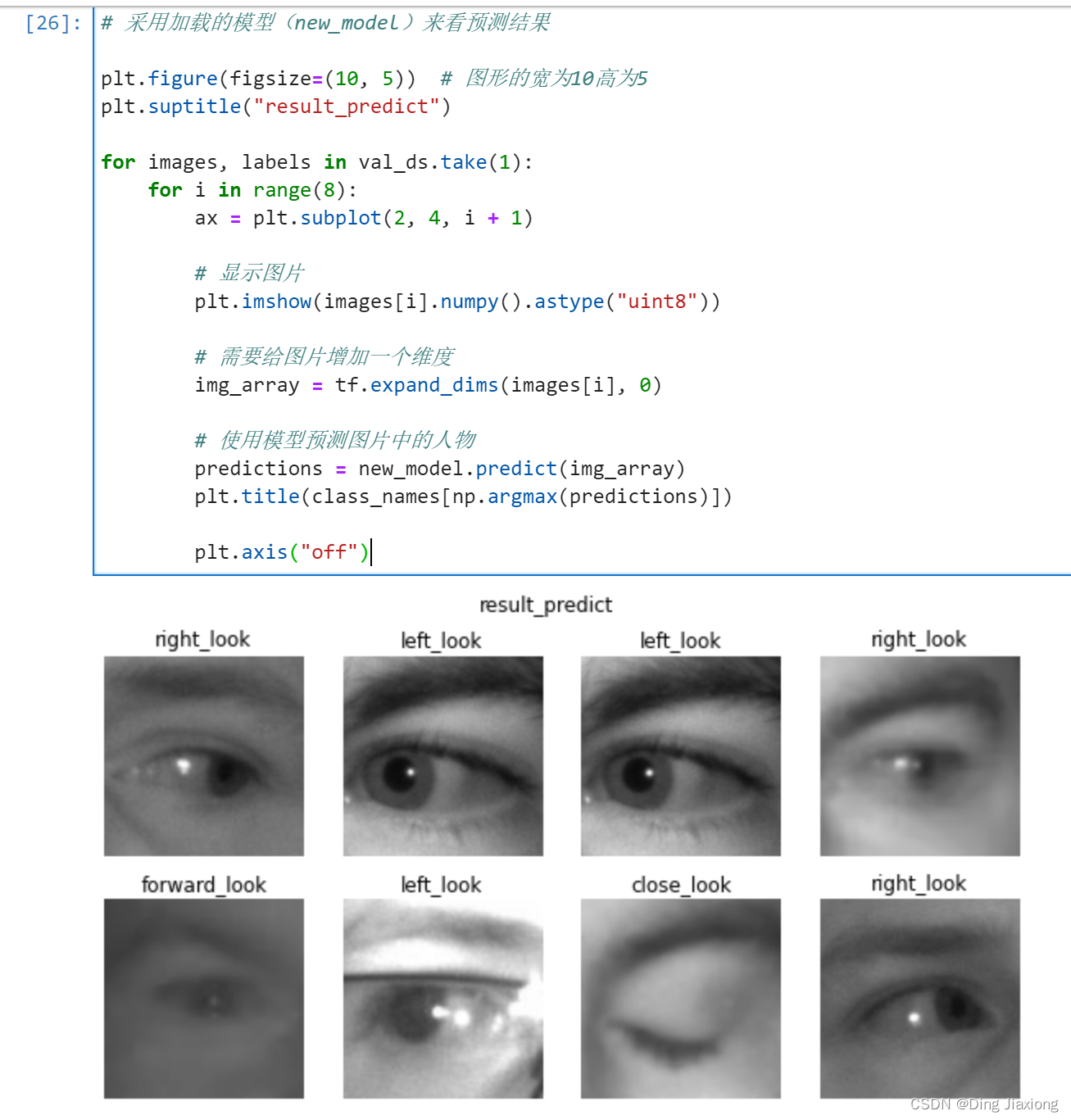
9. 预测
# 采用加载的模型(new_model)来看预测结果

plt.figure(figsize=(10, 5))  # 图形的宽为10高为5
plt.suptitle("result_predict")

for images, labels in val_ds.take(1):
    for i in range(8):
        ax = plt.subplot(2, 4, i + 1)

        # 显示图片
        plt.imshow(images[i].numpy().astype("uint8"))

        # 需要给图片增加一个维度
        img_array = tf.expand_dims(images[i], 0)

        # 使用模型预测图片中的人物
        predictions = new_model.predict(img_array)
        plt.title(class_names[np.argmax(predictions)])

        plt.axis("off")
边栏推荐
- Kotlin算法入门求回文数数算法优化二数字生成规则
- 基于hydra库实现yaml配置文件的读取(支持命令行参数)
- For the first time, I suspect that there is a bug in selenium4 because the iframe element is not found?
- Design of Cluster Gateway in Game Server
- Typescrip编译选项
- Swagger简单使用
- 表达式必须具有与对应表达式相同的数据类型
- 《剑指offer》题解——week3(持续更新)
- dsu on tree(树上启发式合并)学习笔记
- 2022-08-09 顾宇佳 学习笔记
猜你喜欢


随机推荐
gRPC系列(四) 框架如何赋能分布式系统
麒麟V10系统打包Qt免安装包程序
Features of LoRa Chips
表达式必须具有与对应表达式相同的数据类型
刷题错题录2-向上取整、三角形条件、字符串拼接匹配、三数排序思路
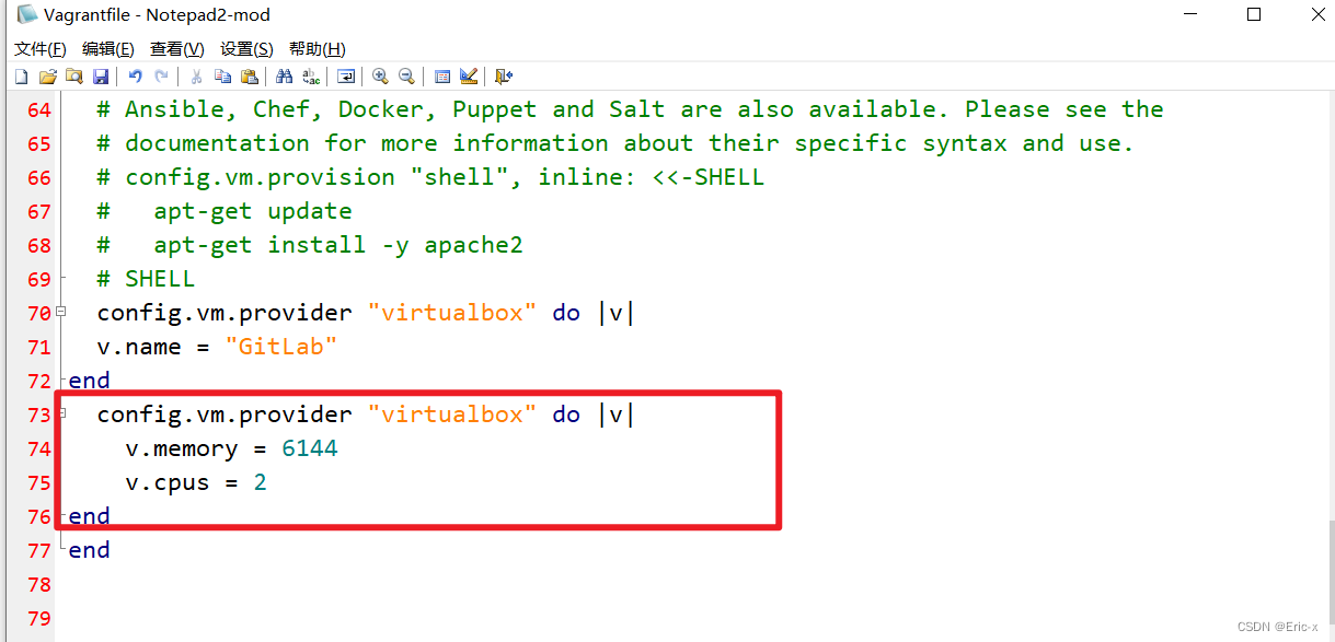
设置Vagrant创建的虚拟机名称和内存
Getting Started with Kotlin Algorithms Calculating Prime Factors
用 Antlr 重构脚本解释器
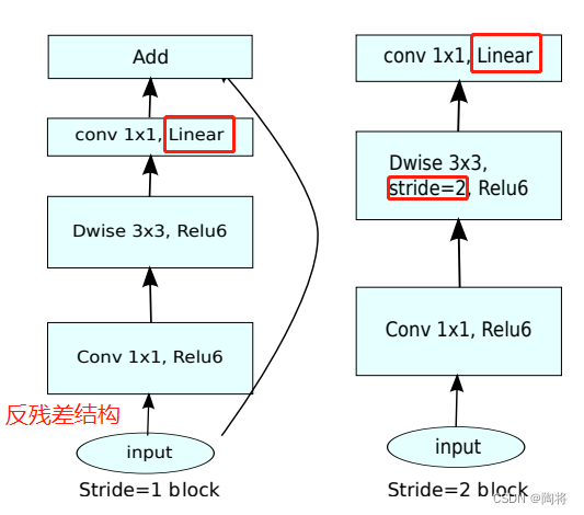
Machine Learning Summary (2)
YTU 2297: KMP pattern matching three (string)
shell之sed
四级独创的阅读词汇表
Creo9.0 特征的成组
Rust从入门到精通06-函数
关于架构的认知
兼容并蓄广纳百川,Go lang1.18入门精炼教程,由白丁入鸿儒,go lang复合容器类型的声明和使用EP04
MySql的索引
【wxGlade学习】wxGlade环境配置
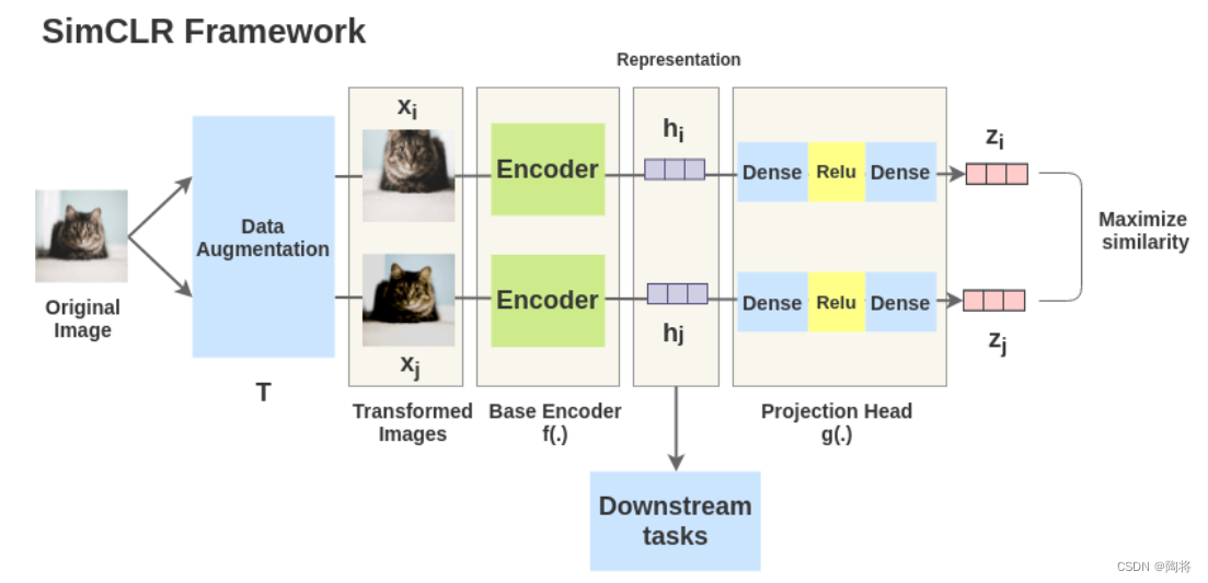
Contrastive Learning Series (3)-----SimCLR
Kotlin算法入门求自由落体