当前位置:网站首页>Principal Component Analysis - Applications of MATLAB in Mathematical Modeling (2nd Edition)
Principal Component Analysis - Applications of MATLAB in Mathematical Modeling (2nd Edition)
2022-08-09 17:18:00 【YuNlear】
数据建模及MATLAB实现(二)
随着信息技术的发展和成熟,各行业积累的数据越来越多,因此需要通过数据建模的方法,从看似杂乱的海量数据中找到有用的信息.
主成分分析(PCA)
在数学建模中,Often study the issue of multiple variables.When the complex relations between variables number and,会显著增加分析问题的复杂性.
为了解决这种问题,Scientists have proposed the principal component analysis(Principal Component Analysis, PCA)的方法.PCA是一种数学降维方法,The main purpose is to originally many has certain correlation variable,Back together for a new set of mutually independent variables.
通常,Mathematical treatment method is to do the original variable linear combination,As a new comprehensive variables.通常,Math will select the first linear combination of the first comprehensive variables to remember F 1 F_1 F1,而 F 1 F_1 F1Need to reflect the original variable information as much as.Information through variance to say,则希望 v a r ( F 1 ) var(F_1) var(F1)尽可能的大,表示 F 1 F_1 F1Contains more information as much as possible.因此 F 1 F_1 F1Should be a linear combination of China's biggest.
And if the first principal component can't represent all variables of information,Requires the second principal component、第三主成分···,While the former existing information do not need to appear in the latter.Using mathematical way is c o v ( F 1 , F 2 ) = 0 cov(F_1,F_2)=0 cov(F1,F2)=0,称 F 2 F_2 F2为第二主成分( c o v ( ) cov() cov()The covariance in math).
Principal component analysis of the typical steps
对原始数据进行标准化处理.
The observation data matrix X X X,有
X = [ x 11 x 12 ⋅ ⋅ ⋅ x 1 p x 21 x 22 ⋅ ⋅ ⋅ x 2 p ⋮ ⋮ ⋱ ⋮ x n 1 x n 2 ⋅ ⋅ ⋅ x n p ] X=\begin{bmatrix} x_{11}&x_{12}&···&x_{1p}\\ x_{21}&x_{22}&···&x_{2p}\\ \vdots&\vdots&\ddots&\vdots\\ x_{n1}&x_{n2}&···&x_{np}\\ \end{bmatrix} X=⎣⎡x11x21⋮xn1x12x22⋮xn2⋅⋅⋅⋅⋅⋅⋱⋅⋅⋅x1px2p⋮xnp⎦⎤
Can be standardized in accordance with the following method to the original data processing:
x i j ∗ = x i j − x j ‾ V a r ( x j ) ( i = 1 , 2 , ⋯ , n ; j = 1 , 2 , ⋯ , p ) x_{ij}^{*}=\frac{x_{ij}-\overline{x_j}}{\sqrt{Var(x_j)}} \ \ \ \ \ \ \ \ (i=1,2,\cdots,n;j=1,2,\cdots,p) xij∗=Var(xj)xij−xj (i=1,2,⋯,n;j=1,2,⋯,p)
其中,
x j ‾ = 1 n Σ n i = 1 x i j ; V a r ( x j ) = 1 n − 1 Σ i = 1 n ( x i j − x j ‾ ) 2 ( j = 1 , 2 , ⋯ , p ) . \overline{x_{j}}=\frac{1}{n}\underset{i=1}{\overset{n}{\Sigma}}x_{ij};Var(x_j)=\frac{1}{n-1}\overset{n}{\underset{i=1}{\Sigma}}(x_ij-\overline{x_j})^2\\ (j=1,2,\cdots,p). xj=n1i=1Σnxij;Var(xj)=n−11i=1Σn(xij−xj)2(j=1,2,⋯,p).计算样本相关系数矩阵.
In the correlation coefficient matrix,Useful to the concept of covariance,See the specific concept百度百科-协方差.And the correlation coefficient is the covariance of standardized values.
R = [ r 11 r 12 ⋯ r 1 p r 21 r 22 ⋯ r 2 p ⋮ ⋮ ⋱ ⋮ r p 1 r p 2 ⋯ r p p ] R= \begin{bmatrix} r_{11}&r_{12}&\cdots&r_{1p}\\ r_{21}&r_{22}&\cdots&r_{2p}\\ \vdots&\vdots&\ddots&\vdots\\ r_{p1}&r_{p2}&\cdots&r_{pp}\\ \end{bmatrix} R=⎣⎡r11r21⋮rp1r12r22⋮rp2⋯⋯⋱⋯r1pr2p⋮rpp⎦⎤
其中,
r i j = c o v ( x i , x j ) = Σ k = 1 n ( x k i − x i ‾ ) ( x k j − x j ‾ ) n − 1 r_{ij}=cov(x_i,x_j)=\frac{\overset{n}{\underset{k=1}{\Sigma}}(x_{ki}-\overline{x_i})(x_{kj}-\overline{x_j})}{n-1} rij=cov(xi,xj)=n−1k=1Σn(xki−xi)(xkj−xj)Calculate the correlation coefficient matrix eigenvalues and corresponding eigenvectors of the
特征值: λ 1 , λ 2 , ⋯ , λ p \lambda_1,\lambda_2,\cdots,\lambda_p λ1,λ2,⋯,λp(Characteristic value namely variance values)
特征向量 a i = ( a i 1 , a i 2 , ⋯ , a i p ) T , i = 1 , 2 , ⋯ , p a_i=(a_{i1},a_{i2},\cdots,a_{ip})^T,i=1,2,\cdots,p ai=(ai1,ai2,⋯,aip)T,i=1,2,⋯,p
选择重要的主成分,并写出主成分表达式
By principal component analysis getp个主成分,But as a result of the variance of the principal component is decreasing,So in the process of practical analysis,Generally not choosep个主成分,But the contribution rate of each principal component cumulative size selection before k k k个主成分.
Contribution is a main component of the proportion of total variance of variance combined:
贡献率 = λ i Σ i = 1 p λ i × 100 % 贡献率=\frac{\lambda_i}{\overset{p}{\underset{i=1}{\Sigma}}\lambda_i}\times100\% 贡献率=i=1Σpλiλi×100%
The greater the contribution,Original variables show that the principal component contains the more information.一般kA principal components need the cumulative contribution rate in80%或85%以上,In order to ensure comprehensive variables can include the original most of the information.计算主成分得分
According to the standardization of original data,According to the sample,Each generation in the component expressions,You can get under the main component of each sample of new data,The principal component scores.具体形式如下:
[ F 11 F 12 ⋯ F 1 k F 21 F 22 ⋯ F 2 k ⋮ ⋮ ⋱ ⋮ F n 1 F n 2 ⋯ F n k ] \begin{bmatrix} F_{11}&F_{12}&\cdots&F_{1k}\\ F_{21}&F_{22}&\cdots&F_{2k}\\ \vdots&\vdots&\ddots&\vdots\\ F_{n1}&F_{n2}&\cdots&F_{nk}\\ \end{bmatrix} ⎣⎡F11F21⋮Fn1F12F22⋮Fn2⋯⋯⋱⋯F1kF2k⋮Fnk⎦⎤
主成分分析MATLAB程序设计
The following analysis of main componentMATLAB程序PCA.m
function [F,new_score]=PCA(A,T)
a=size(A,1);
b=size(A,2);
% 数据标准化处理
for i=1:b
    SA(:,i)=(A(:,i)-mean(A(:,i)))/std(A(:,i));
end
% Calculate the correlation coefficient matrix eigenvalues and corresponding eigenvectors
CM=corrcoef(SA);
[V,D]=eig(CM);
for j=1:b
    DS(j,1)=D(b+1-j,b+1-j);
end
for i=1:b
    DS(i,2)=DS(i,1)/sum(DS(:,1));
    DS(i,3)=sum(DS(1:i,2));
end
%保留k个主成分
for K=1:b
    if(DS(K,3)>=T)
        Com_num=K;
        brek;
    end
end
%提取主成分对应的特征向量
for i=1:Com_num
    F(:,i)=V(:,b+1-i);
end
new_score=SA*F;
边栏推荐
- 【深度学习】原始问题和对偶问题(六)
- Faster R-CNN 论文总结
- hugging face tutorial - Chinese translation - preprocessing
- Stetman读peper小记:Defense-Resistant Backdoor Attacks Against DeepNeural Networks in Outsourced Cloud
- 【深度学习】全面理解支持向量机SVM(七)
- Vim实用技巧_1.vim解决问题的方式
- 将类指针强制转换为void*指针进行传参的使用方法
- 嵌入式三级笔记
- Postgraduate Work Weekly (Week 6)
- 【力扣】662. 二叉树最大宽度
猜你喜欢

【研究生工作周报】(第十二周)

flask局域网访问失败解决方法(使用pycharm运行代码的一定要看)

Markdown 文档生成 PDF

The experience of using Photoshop CS6

Vim实用技巧_4.管理多个文件(打开 + 切分 + 保存 + netrw)
![[Deep Learning] SVM solves the linear inseparable situation (8)](/img/3c/199f3ff3fb0546bcd7f70bd71030a0.png)
[Deep Learning] SVM solves the linear inseparable situation (8)
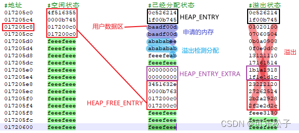
堆(heap)系列_0x07:NT堆调试支持_滞后发现调试支持

【深度学习】模型选择、欠/过拟合和感受野(三)
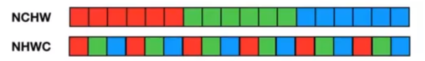
tensor转cv::Mat(即CHW转HWC)原理含C#代码实现

【深度学习】归一化(十一)
随机推荐
深入浅出最优化(6) 最小二乘问题的特殊方法
灰色关联度矩阵——MATLAB在数学建模中的应用
hugging face tutorial - Chinese translation - model summary
【Postgraduate Work Weekly】(Week 9)
[Paper reading] LIME: Low-light Image Enhancement via Illumination Map Estimation (the most complete notes)
【研究生工作周报】(第三周)
【深度学习】原始问题和对偶问题(六)
抱抱脸(hugging face)教程-中文翻译-对预先训练过的模特进行微调
【工具使用】Modscan32软件使用详解
【深度学习】梯度下降与梯度爆炸(十)
hugging face tutorial - Chinese translation - share a model
【力扣】17. 电话号码的字母组合
VGG pytorch实现
【深度学习】SVM解决线性不可分情况(八)
【深度学习】全面理解支持向量机SVM(七)
蓝桥杯嵌入式备赛
人脸识别示例代码解析(二)——人脸识别解析
交叉编译 OpenSSL
【知识分享】知识链路-Modbus通信知识链路
Candide3 face animation model