Wu Enda's machine learning assignment -- Logical Regression

1 Logistic regression

In this part of the exercise , You will build a logistic regression model to predict whether a student can enter college . Suppose you are an administrator of a University , Based on the results of the two exams , To decide whether each applicant is admitted . You have historical data on previous Applicants , It can be used as a logistic regression training set . For each training sample , You have the scores of the applicant's two evaluations and the results of admission . To accomplish this prediction task , We are going to build a classification model that can evaluate the possibility of admission based on two test scores .

1.1 Visualizing the data

Before starting to implement the algorithm , It is best to visualize the data
Add library

import pandas as pd
import matplotlib.pyplot as plt
import numpy as np
from sklearn.metrics import classification_report

Read training set data

path = 'ex2data1.txt'
data = pd.read_csv(path, header=None, names=['exam 1 score', 'exam 2 score', 'admitted'])
# print(data.head())
# print(data.describe())

Draw the positive and negative classes in the form of scatter diagram

#  Separate admission and non admission data 
positive = data[data.admitted.isin(['1'])]
negative = data[data.admitted.isin(['0'])]

#  Visual training set data 
fig, ax = plt.subplots(figsize=(6, 5))
ax.scatter(positive['exam 1 score'], positive['exam 2 score'], c='black', marker='+', label='admitted')
ax.scatter(negative['exam 1 score'], negative['exam 2 score'], c='yellow', marker='o', label='not admitted')
ax.legend(loc=2)  #  Data point notes 
ax.set_xlabel('exam 1 score')
ax.set_ylabel('exam 2 score')
ax.set_title('trainging data')

1.2 sigmoid function

def sigmoid(x):
    return np.exp(x) / (1 + np.exp(x))

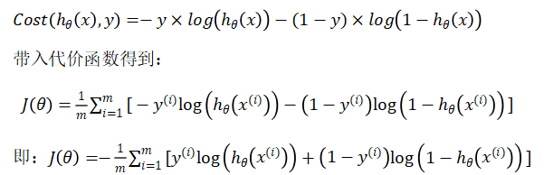
1.3 Cost function

def computecost(X, y, theta):
    theta = np.matrix(theta)
    X = np.matrix(X)
    y = np.matrix(y)
    first = np.multiply(-y, np.log(sigmoid(np.dot(X, theta.T))))
    second = np.multiply((1 - y), np.log(1 - sigmoid(np.dot(X, theta.T))))
    return np.sum(first - second) / (len(X))

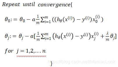
1.4 gradient descent

def gradientdescent(X, y, theta, alpha, epoch):
    temp = np.matrix(np.zeros(theta.shape))
    m = X.shape[0]
    cost = np.zeros(epoch)

    for i in range(epoch):
        A = sigmoid(np.dot(X, theta.T))
        temp = theta - (alpha / m) * (A - y).T * X
        theta = temp
        cost[i] = computecost(X, y, theta)

    return theta, cost

1.5 Training theta Parameters

Before training, normalize the students' scores

data.insert(0, 'Ones', 100)
cols = data.shape[1]  #  Number of columns 
X = data.iloc[:, 0:cols - 1]
y = data.iloc[:, cols - 1:cols]
# theta = np.zeros(X.shape[1])
theta = np.ones(3)
X = np.matrix(X)
X = X / 100  #  normalization 
y = np.matrix(y)
theta = np.matrix(theta)

Training begins

alpha = 0.3
epoch = 100000
origin_cost = computecost(X, y, theta)
final_theta, cost = gradientdescent(X, y, theta, alpha, epoch)

Output theta Parameters

print(final_theta)
# [[-24.99361363 20.48877093 20.01095566]]

1.6 Evaluation algorithm

Prediction function , Enter student grades , Output the probability of admission

def predict(theta, X):
    probability = sigmoid(np.dot(X, theta.T))
    return [1 if x >= 0.5 else 0 for x in probability]

Check the accuracy

predictions = predict(final_theta, X)
correct = [1 if a == b else 0 for (a, b) in zip(predictions, y)]
accuracy = sum(correct) / len(X)
print(accuracy)
#  Output  0.89

Or use sklearn To test

from sklearn.metrics import classification_report
print(classification_report(predictions, y))

              precision    recall  f1-score   support

           0       0.85      0.87      0.86        39
           1       0.92      0.90      0.91        61

    accuracy                           0.89       100
   macro avg       0.88      0.89      0.88       100
weighted avg       0.89      0.89      0.89       100

The cost function changes

fig, ax = plt.subplots()
ax.plot(np.arange(epoch), cost, 'r')
ax.set_xlabel('Iterations')
ax.set_ylabel('Cost')
ax.set_title('Cost vs. Training Epoch')
plt.show()

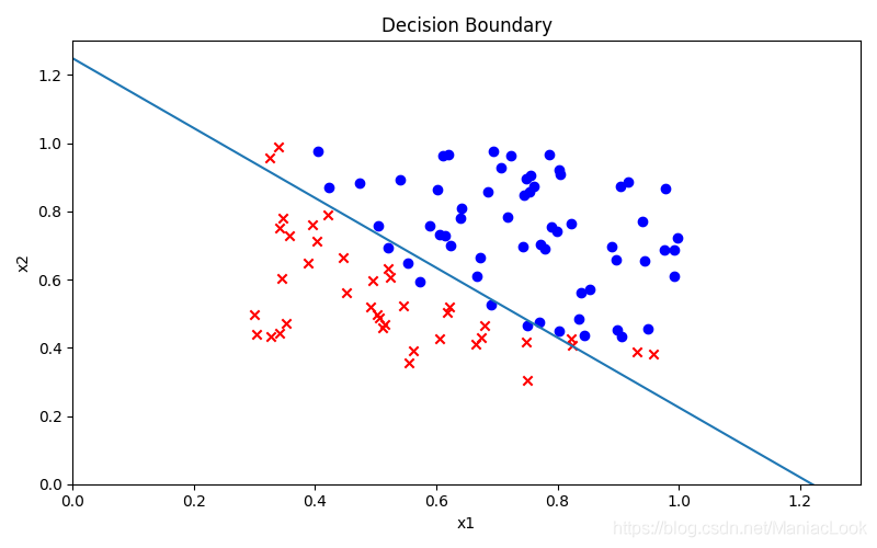
1.7 Decision boundaries

x1 = np.arange(1.3, step=0.01)
x2 = -(final_theta[0, 0] + x1 * final_theta[0, 1]) / final_theta[0, 2]

fig, ax = plt.subplots(figsize=(8, 5))
ax.scatter(positive['exam 1 score'] / 100, positive['exam 2 score'] / 100, c='b', label='Admitted')
ax.scatter(negative['exam 1 score'] / 100, negative['exam 2 score'] / 100, c='r', marker='x', label='Not Admitted')
ax.plot(x1, x2)
ax.set_xlim(0, 1.3)
ax.set_ylim(0, 1.3)
ax.set_xlabel('x1')
ax.set_ylabel('x2')
ax.set_title('Decision Boundary')
plt.show()

Decision boundary diagram

2 Regularized logistic regression

In this part of the exercise , You will implement regularized logistic regression , To predict whether the microchip of the manufacturer passes the quality assurance （QA）. stay QA In the process , Every microchip has to go through various tests , To make sure it works .
Suppose you are the product manager of the factory , You did two different tests on the test results of some microchips . From these two tests , Whether you want to accept microchip or whether you want to reject microchip . To help you make a decision , You have a data set of past chip test results , From which you can build a logistic regression model .

2.1 Visualizing the data

First read the training set

data = pd.read_csv('ex2data2.txt', names=['Test 1', 'Test 2', 'Accepted'])
print(data.head())
print(data.describe())

Output results

     Test 1   Test 2  Accepted
0  0.051267  0.69956         1
1 -0.092742  0.68494         1
2 -0.213710  0.69225         1
3 -0.375000  0.50219         1
4 -0.513250  0.46564         1
           Test 1      Test 2    Accepted
count  118.000000  118.000000  118.000000
mean     0.054779    0.183102    0.491525
std      0.496654    0.519743    0.502060
min     -0.830070   -0.769740    0.000000
25%     -0.372120   -0.254385    0.000000
50%     -0.006336    0.213455    0.000000
75%      0.478970    0.646562    1.000000
max      1.070900    1.108900    1.000000

Then draw a picture

#  data classification 
positive = data[data.Accepted.isin(['1'])]
negative = data[data.Accepted.isin(['0'])]

#  Visualization data 
fig, ax = plt.subplots(figsize=(6, 4))
ax.scatter(positive['Test 1'], positive['Test 2'], c='black', marker='+', label='y=1')
ax.scatter(negative['Test 1'], negative['Test 2'], c='yellow', marker='o', label='y=0')
ax.legend(loc=1)
ax.set_xlabel('Microchip Test 1')
ax.set_ylabel('Microchip Test 2')
ax.set_title('Plot of training data')
plt.show()

2.2 Feature mapping

One way to better fit the data is to create more features from each data point . We will map features to x1 and x2 All polynomial terms of , Until the sixth power . Computation (1 + x1 + x2 + x1² + x1x2 + x2² + … + x1x2⁵ + x2⁶)

#  Feature mapping 
def feature_mapping(x1, x2, power):
    data2 = {
    }
    for i in np.arange(power + 1):
        for p in np.arange(i + 1):
            data2["f{}{}".format(i - p, p)] = np.power(x1, i - p) * np.power(x2, p)
    return pd.DataFrame(data2)


#  Calculation 6 Characteristic mapping of order 
x1 = data['Test 1'].values
x2 = data['Test 2'].values
data2 = feature_mapping(x1, x2, 6)
print(data2.head())

   f00       f10      f01       f20  ...       f33       f24       f15       f06
0  1.0  0.051267  0.69956  0.002628  ...  0.000046  0.000629  0.008589  0.117206
1  1.0 -0.092742  0.68494  0.008601  ... -0.000256  0.001893 -0.013981  0.103256
2  1.0 -0.213710  0.69225  0.045672  ... -0.003238  0.010488 -0.033973  0.110047
3  1.0 -0.375000  0.50219  0.140625  ... -0.006679  0.008944 -0.011978  0.016040
4  1.0 -0.513250  0.46564  0.263426  ... -0.013650  0.012384 -0.011235  0.010193

As a result of this mapping , Our two eigenvectors （ Two QA Test score ） Converted to 28 Dimension vector . Trained on this high-dimensional eigenvector logistic Regression classifiers will have more complex decision boundaries , And there will be nonlinearity when drawing in our two-dimensional diagram .
Although feature mapping allows us to build more expressive classifiers , But it's also easier to over fit . In the next part of the exercise , You will implement regularization logistic Regression to fit the data , We'll also see for ourselves how regularization can help solve the over fitting problem .

2.3 Cost function and gradient

Now implement the code to compute the regular logistic The cost function and gradient of regression .
Think about it ,logistic The regularization cost function in regression is

Please note that , Parameters should not be regularized θ0.
The gradient of the cost function is a vector , Among them the first j The elements are defined as follows ：

# sigmoid  function 
def sigmoid(x):
    return 1 / (1 + np.exp(-x))


#  Cost function 
def cost(theta, X, y):
    first = (-y) * np.log(sigmoid(X @ theta))
    second = (1 - y) * np.log(1 - sigmoid(X @ theta))
    return np.mean(first - second)


#  Regularization cost function 
def costreg(theta, X, y, learningrate):
    _theta = theta[1:]
    reg = (learningrate / (2 * len(X))) * (_theta @ _theta)
    return cost(theta, X, y) + reg

#  gradient 
def gradient(theta, X, y):
    return (X.T @ (sigmoid(X @ theta) - y)) / len(X)


#  Regularized gradient 
def gradientreg(theta, X, y, learningrate):
    reg = (learningrate / len(X)) * theta
    reg[0] = 0  #  No punishment θ0
    return gradient(theta, X, y) + reg

2.4 Training parameters θ

Get the training set and initialize θ by 0

X = data2.values
y = data['Accepted'].values
theta = np.zeros(X.shape[1])
print(X.shape, y.shape, theta.shape)
print(costreg(theta, X, y, 1))

(118, 28) (118,) (28,)
0.6931471805599454

（1） use fmin_tnc Function training

result1 = opt.fmin_tnc(func=costreg, x0=theta, fprime=gradientreg, args=(X, y, 2))
print(result1)

(array([ 1.02253248,  0.56283944,  1.13465456, -1.78529748, -0.66539169,
       -1.01863181,  0.13957059, -0.29358911, -0.30102279, -0.08324363,
       -1.27205982, -0.06137378, -0.53996494, -0.17881798, -0.94198718,
       -0.14054843, -0.17736659, -0.07697368, -0.22918936, -0.21349659,
       -0.37205336, -0.86417647,  0.00890082, -0.26795949, -0.0036225 ,
       -0.28315229, -0.07321593, -0.75992548]), 57, 1)

（2） use minimize Function training

result2 = opt.minimize(fun=costreg, x0=theta, args=(X, y, 2), method='TNC', jac=gradientreg)
print(result2)

fun: 0.5830356764058148
     jac: array([0.00318613, 0.00371841, 0.01438163, 0.00439174, 0.0042439 ,
       0.01363881, 0.0025095 , 0.00300901, 0.00121719, 0.01128844,
       0.00351398, 0.00083453, 0.00220748, 0.00131178, 0.0112205 ,
       0.00258022, 0.00113796, 0.00020022, 0.0017479 , 0.00077718,
       0.00942953, 0.00305894, 0.00032368, 0.0007994 , 0.00012105,
       0.00142873, 0.00056985, 0.00951201])
 message: 'Converged (|f_n-f_(n-1)| ~= 0)'
    nfev: 57
     nit: 2
  status: 1
 success: True
       x: array([ 1.02253248,  0.56283944,  1.13465456, -1.78529748, -0.66539169,
       -1.01863181,  0.13957059, -0.29358911, -0.30102279, -0.08324363,
       -1.27205982, -0.06137378, -0.53996494, -0.17881798, -0.94198718,
       -0.14054843, -0.17736659, -0.07697368, -0.22918936, -0.21349659,
       -0.37205336, -0.86417647,  0.00890082, -0.26795949, -0.0036225 ,
       -0.28315229, -0.07321593, -0.75992548])

2.5 Evaluating logistic regression

final_theta = result1[0]
predictions = predict(final_theta, X)
correct = [1 if a == b else 0 for (a, b) in zip(predictions, y)]
accuracy = sum(correct) / len(X)
print(accuracy)

final_theta = result2.x
predictions = predict(final_theta, X)
correct = [1 if a == b else 0 for (a, b) in zip(predictions, y)]
accuracy = sum(correct) / len(X)
print(accuracy)

from sklearn.metrics import classification_report
print(classification_report(y, predictions))

0.8050847457627118
0.8050847457627118

              precision    recall  f1-score   support

           0       0.85      0.75      0.80        60
           1       0.77      0.86      0.81        58

    accuracy                           0.81       118
   macro avg       0.81      0.81      0.80       118
weighted avg       0.81      0.81      0.80       118

2.6 Decision boundaries

x = np.linspace(-1, 1.5, 250)
xx, yy = np.meshgrid(x, x)

z = feature_mapping(xx.ravel(), yy.ravel(), 6).values
z = z @ final_theta
z = z.reshape(xx.shape)

fig, ax = plt.subplots()
ax.scatter(positive['Test 1'], positive['Test 2'], c='black', marker='+', label='y=1')
ax.scatter(negative['Test 1'], negative['Test 2'], c='yellow', marker='o', label='y=0')
ax.legend(loc=1)
ax.set_xlabel('Microchip Test 1')
ax.set_ylabel('Microchip Test 2')
ax.set_title('Plot of training data')
plt.contour(xx, yy, z, 0)  #  contour 
plt.ylim(-0.8, 1.2)
plt.show()

The following figure for $\lambda$ = 2 The decision boundary of

$\lambda$ = 0 when

$\lambda$ = 100 when