当前位置:网站首页>核方法 Kernel method
核方法 Kernel method
2022-08-11 05:35:00 【Pr4da】
1.内积(点积)
内积,又叫做点积,数量积或标量积。假设存在两个向量 a = [ a 1 , a 2 , . . . , a n ] a=[a_{1}, a_{2}, ..., a_{n}] a=[a1,a2,...,an]和 b = [ b 1 , b 2 , . . . , b n ] b=[b_{1},b_{2},...,b_{n}] b=[b1,b2,...,bn],内积的计算方法为:
a ⋅ b = a 1 b 1 + a 2 b 2 + ⋯ + a n b n a\cdot b= a_{1}b_{1}+a_{2}b_{2}+\cdots +a_{n}b_{n} a⋅b=a1b1+a2b2+⋯+anbn
2.核方法 1
核方法的主要思想是基于这样一个假设:“在低维空间中不能线性分割的点集,通过转化为高维空间中的点集时,很有可能变为线性可分的” ,例如有两类数据,一类为 x < a ∪ x > b x<a\cup x>b x<a∪x>b;另一部分为 a < x < b a<x<b a<x<b。要想在一维空间上线性分开是不可能的。然而我们可以通过F(x)=(x-a)(x-b)把一维空间上的点转化到二维空间上,这样就可以划分两类数据 F ( x ) > 0 F(x)>0 F(x)>0, F ( x ) < 0 F(x)<0 F(x)<0;从而实现线性分割。如下图所示: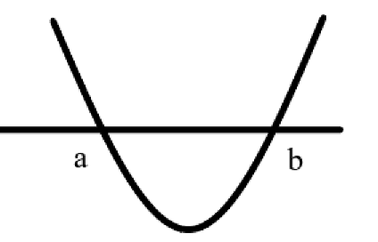
定义一个核函数 K ( x 1 , x 2 ) = * ϕ ( x 1 ) , ϕ ( x 2 ) * K(x_{1},x_{2})=\left \langle \phi (x_{1}),\phi (x_{2})\right \rangle K(x1,x2)=*ϕ(x1),ϕ(x2)*, 其中 x 1 x_{1} x1和 x 2 x_{2} x2是低维度空间中的点(在这里可以是标量,也可以是向量), ϕ ( x i ) \phi (x_{i}) ϕ(xi)是低维度空间的点转化为高维度空间中的点的表示, * , * \left \langle ,\right \rangle *,*表示向量的内积。这里核函数的表达方式一般都不会显式地写为内积的形式,即我们不关心高维度空间的形式。
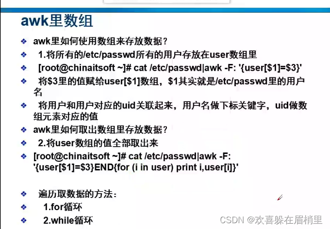
这里有个很重要的问题,就是我们为什么要关心内积。一般的我们可以把分类或回归问题分为两类:参数学习和基于实例的学习。参数学习就是通过一堆训练数据把模型的参数学习出来,训练完成之后训练数据就没有用了,新数据使用已经训练好的模型进行预测,例如人工神经网络。而基于实例的学习(又叫基于内存的学习)是在预测的时候会使用训练数据,例如KNN算法,会计算新样本与训练样本的相似度。计算相似度一般通过向量的内积来表示。从这里可以看出,核方法不是万能的,它一般只针对基于实例的学习。
3.核方法的定义和例子2
给定一个映射关系 ϕ \phi ϕ,我们定义相应的核函数为:
K ( x , y ) = ϕ ( x ) T ϕ ( y ) K(x,y)=\phi (x)^{T}\phi (y) K(x,y)=ϕ(x)Tϕ(y)
则内积运算 < ϕ ( x ) , ϕ ( y ) > <\phi (x), \phi (y)> <ϕ(x),ϕ(y)>可以用核 K ( x , y ) K(x,y) K(x,y)来表示。
例如,给定两个 n n n维向量 x x x和 y y y, x , y ∈ R n x,y\in \mathbb{R}^{n} x,y∈Rn,我们定义一个核函数 K ( x , y ) = ( x T y ) 2 K(x,y)=(x^{T}y)^{2} K(x,y)=(xTy)2,将该二次多项式展开会得到如下表达式: ( x 1 y 1 + . . . + x n y n ) 2 (x_{1}y_{1}+...+x_{n}y_{n})^{2} (x1y1+...+xnyn)2。
但 K ( x , y ) K(x,y) K(x,y)还可以写成:
KaTeX parse error: No such environment: align at position 8: \begin{̲a̲l̲i̲g̲n̲}̲ K(x,y)&=(x^{T}…
如果 n n n为2的话,即 x T = ( x 1 , x 2 ) x^{T}=(x_{1},x_{2}) xT=(x1,x2), y T = ( y 1 , y 2 ) y^{T}=(y_{1},y_{2}) yT=(y1,y2)。若直接对 ( x T y ) 2 (x^{T}y)^{2} (xTy)2进行计算
( x T y ) 2 = ( x 1 y 1 + x 2 y 2 ) 2 = ( x 1 y 1 ) 2 + 2 x 1 y 1 x 2 y 2 + ( x 2 y 2 ) 2 (x^{T}y)^{2}=(x_{1}y_{1}+x_{2}y_{2})^{2}=(x_{1}y_{1})^{2}+2x_{1}y_{1}x_{2}y_{2}+(x_{2}y_{2})^{2} (xTy)2=(x1y1+x2y2)2=(x1y1)2+2x1y1x2y2+(x2y2)2
如果我们先对 x x x和 y y y进行映射, ϕ ( x ) \phi(x) ϕ(x)可以将 x x x映射为:
ϕ ( x ) = [ x 1 x 1 x 1 x 2 x 2 x 1 x 2 x 2 ] \phi (x)=\begin{bmatrix} x_{1}x_{1}\\ x_{1}x_{2}\\ x_{2}x_{1}\\ x_{2}x_{2}\\ \end{bmatrix} ϕ(x)=⎣⎢⎢⎡x1x1x1x2x2x1x2x2⎦⎥⎥⎤
ϕ ( y ) \phi(y) ϕ(y)可以将 y y y映射为:
ϕ ( y ) = [ y 1 y 1 y 1 y 2 y 2 y 1 y 2 y 2 ] \phi (y)=\begin{bmatrix} y_{1}y_{1}\\ y_{1}y_{2}\\ y_{2}y_{1}\\ y_{2}y_{2}\\ \end{bmatrix} ϕ(y)=⎣⎢⎢⎡y1y1y1y2y2y1y2y2⎦⎥⎥⎤
然后再对 ϕ ( x ) \phi (x) ϕ(x)和 ϕ ( y ) \phi (y) ϕ(y)进行内积运算:
< ϕ ( x ) , ϕ ( y ) > = ( x 1 y 1 ) 2 + 2 x 1 x 2 y 1 y 2 + ( x 2 y 2 ) 2 <\phi (x), \phi (y)>=(x_{1}y_{1})^{2}+2x_{1}x_{2}y_{1}y_{2}+(x_{2}y_{2})^{2} <ϕ(x),ϕ(y)>=(x1y1)2+2x1x2y1y2+(x2y2)2
我们发现结果和直接展开运算一样,但是直接展开经过了一次平方运算,复杂度为 O ( n 2 ) O(n^{2}) O(n2),而经过映射之后只需一次内积运算,复杂度为 O ( n ) O(n) O(n),大大提高了效率。
再比如,对于核函数:
KaTeX parse error: No such environment: align at position 8: \begin{̲a̲l̲i̲g̲n̲}̲ K(x,y)&=(x^{T}…
同上,若 x x x和 y y y均为二维向量,则映射函数为:
ϕ = [ x 1 x 1 x 1 x 2 x 2 x 1 x 2 x 2 2 c x 1 2 c x 2 ] \phi =\begin{bmatrix} x_{1}x_{1}\\ x_{1}x_{2}\\ x_{2}x_{1}\\ x_{2}x_{2}\\ \sqrt{2c}x_{1}\\ \sqrt{2c}x_{2}\\ \end{bmatrix} ϕ=⎣⎢⎢⎢⎢⎢⎢⎡x1x1x1x2x2x1x2x22cx12cx2⎦⎥⎥⎥⎥⎥⎥⎤
从多项式可以看到,参数 c c c控制着一阶和二阶多项式的权重。如果将二阶多项式推广到 d d d阶,则核函数 K ( x , y ) = ( x T y + c ) d K(x,y)=(x^{T}y+c)^{d} K(x,y)=(xTy+c)d会将原来的向量映射到 ( n + d d ) \begin{pmatrix} n+d\\ d\\\end{pmatrix} (n+dd)维,尽管在该空间中的复杂度为 O ( n d ) O(n^{d}) O(nd),但经过$\phi 映 射 后 计 算 复 杂 度 为 映射后计算复杂度为 映射后计算复杂度为O(n)$。
4. 常见的核方法
常见的三种核方法:
线性核(Linear kernel): K ( x , y ) = x T y K(x,y)=x^{T}y K(x,y)=xTy
径向基核(Radial basis function kernel, RBF kernel): K ( x , y ) = e x p ( − γ ∥ x − y ∥ 2 ) K(x,y)=exp(-\gamma \left \| x-y\right \|^{2}) K(x,y)=exp(−γ∥x−y∥2)
d d d次多项式核(Polynomial kernel): K ( x , y ) = ( x T y + c ) d K(x,y)=(x^{T}y+c)^{d} K(x,y)=(xTy+c)d
下面我们依次使用这些核函数对非线性问题进行分类,如下图所示,有两个待分类标签,显然他们在二维空间是线性不可分的,我们需要使用核函数把它们映射到更高维空间中,让它们线性可分。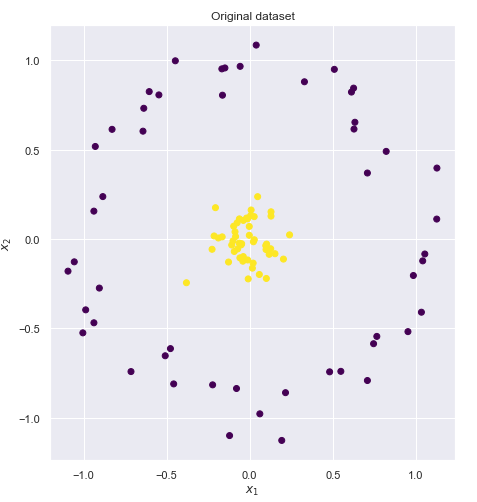
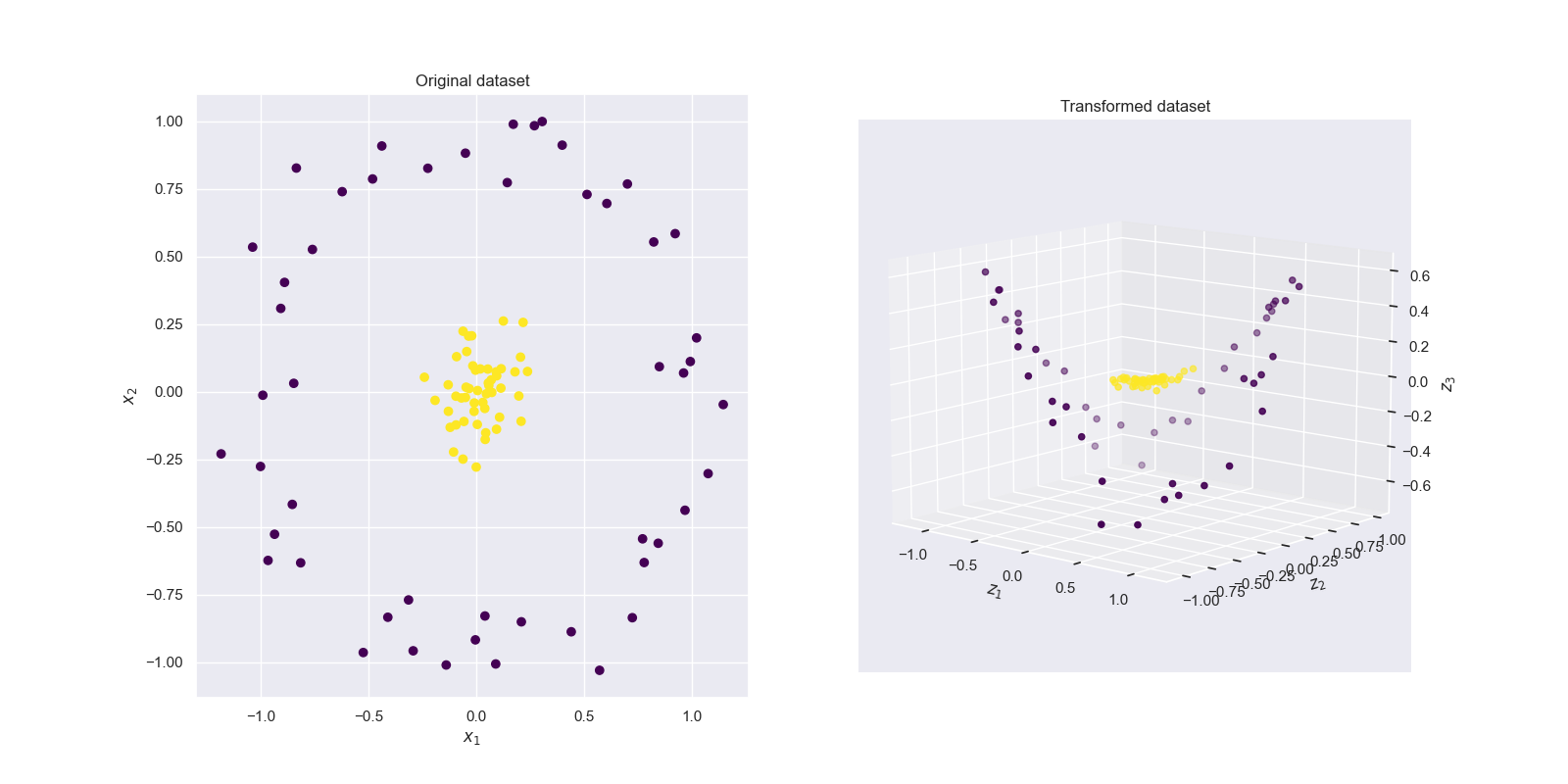
4.1 线性核
核函数:
K ( x , y ) = x T y K(x,y)=x^{T}y K(x,y)=xTy
令 x = ( x 1 , x 2 ) T x=(x_{1},x_{2})^{T} x=(x1,x2)T, y = ( y 1 , y 2 ) T y=(y_{1},y_{2})^{T} y=(y1,y2)T,即维度为2,我们得到:
KaTeX parse error: No such environment: align at position 8: \begin{̲a̲l̲i̲g̲n̲}̲ K(\begin{pmatr…
可以看到线性核的映射 ϕ ( x ) \phi (x) ϕ(x)就是 x x x本身。
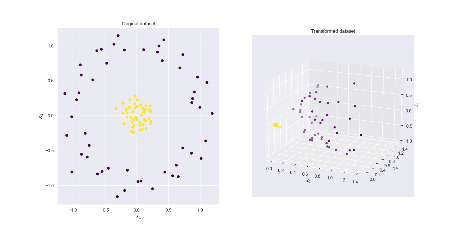
代码:
import numpy as np
import pandas as pd
import seaborn as sns
from matplotlib import pyplot as plt
from mpl_toolkits.mplot3d import Axes3D
from mpl_toolkits import mplot3d
from IPython.display import HTML, Image

%matplotlib inline
sns.set()

from sklearn.datasets import make_circles

def feature_map_1(X):
    return np.asarray((X[:,0], X[:,1], X[:,0]*X[:,1])).T

X, y = make_circles(100, factor=.1, noise=.1)
Z = feature_map_1(X)

#2D scatter plot
fig = plt.figure(figsize = (16,8))
ax = fig.add_subplot(1, 2, 1)
ax.scatter(X[:,0], X[:,1], c = y, cmap = 'viridis')
ax.set_xlabel('$x_1$')
ax.set_ylabel('$x_2$')
ax.set_title('Original dataset')

#3D scatter plot
ax = fig.add_subplot(1, 2, 2, projection='3d')
ax.scatter3D(Z[:,0],Z[:,1], Z[:,2],c = y, cmap = 'viridis' ) #,rstride = 5, cstride = 5, cmap = 'jet', alpha = .4, edgecolor = 'none' )
ax.set_xlabel('$z_1$')
ax.set_ylabel('$z_2$')
ax.set_zlabel('$z_3$')
ax.set_title('Transformed dataset')
我们将线性核函数映射后的数据可视化,得到的结果如图3所示,但从结果发现,线性映射之后的数据点仍然不是线性可分的。
4.2 多项式核
二维二阶多项式核函数: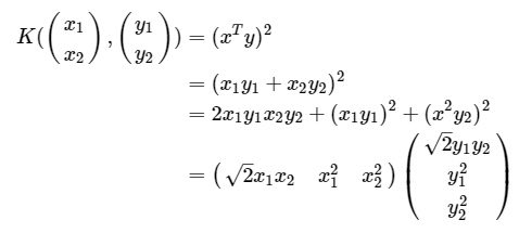
因此, ϕ ( ( x 1 x 2 ) ) = ( 2 x 1 x 2 x 1 2 x 2 2 ) \phi (\begin{pmatrix} x_{1}\\ x_{2} \\ \end{pmatrix})=\begin{pmatrix} \sqrt{2}x_{1}x_{2}\\ x_{1}^{2}\\ x_{2}^{2}\\ \end{pmatrix} ϕ((x1x2))=⎝⎛2x1x2x12x22⎠⎞
画出经二阶多项式映射后的数据分布:
import numpy as np
import pandas as pd
import seaborn as sns
from matplotlib import pyplot as plt
from mpl_toolkits.mplot3d import Axes3D
from mpl_toolkits import mplot3d
from IPython.display import HTML, Image

#%matplotlib inline
sns.set()

from sklearn.datasets import make_circles

def feature_map_0(X):
    return np.asarray((X[:,0]**2, X[:,1]**2, np.sqrt(2)*X[:,0]*X[:,1])).T

X, y = make_circles(100, factor=.1, noise=.1)
Z = feature_map_0(X)

#2D scatter plot
fig = plt.figure(figsize = (16,8))
ax = fig.add_subplot(1, 2, 1)
ax.scatter(X[:,0], X[:,1], c = y, cmap = 'viridis')
ax.set_xlabel('$x_1$')
ax.set_ylabel('$x_2$')
ax.set_title('Original dataset')

#3D scatter plot
ax = fig.add_subplot(1, 2, 2, projection='3d')
ax.scatter3D(Z[:,0],Z[:,1], Z[:,2],c = y, cmap = 'viridis' ) #,rstride = 5, cstride = 5, cmap = 'jet', alpha = .4, edgecolor = 'none' )
ax.set_xlabel('$z_1$')
ax.set_ylabel('$z_2$')
ax.set_zlabel('$z_3$')
ax.set_title('Transformed dataset')
本文原载于我的简书。
参考
边栏推荐
- 阿里巴巴规范之POJO类中布尔类型的变量都不要加is前缀详解
- buildroot嵌入式文件系统中vi显示行号
- iptables入门
- ETCD cluster fault emergency recovery - local data is available
- deepin v20.6+cuda+cudnn+anaconda(miniconda)
- HCIP OSPF/MGRE综合实验
- Threatless Technology-TVD Daily Vulnerability Intelligence-2022-8-2
- Es common operations and classical case
- HCIP OSPF动态路由协议
- Numpy_备注
猜你喜欢

随机推荐
Solve the problem that port 8080 is occupied
SSH服务详解
华为防火墙会话 session table
window7开启远程桌面功能
Threatless Technology-TVD Daily Vulnerability Intelligence-2022-8-2
八股文之jvm
(3) Software testing theory (understanding the knowledge of software defects)
cloudreve使用体验
HCIP实验(pap、chap、HDLC、MGRE、RIP)
CLUSTER DAY02 (Keepalived Hot Standby, Keepalived+LVS, HAProxy Server)
利用opencv读取图片,重命名。
visio文件批量转pdf
查看可执行文件依赖的库ldd
ansible batch install zabbix-agent
mysql数据库安装教程(超级超级详细)
FusionCompute8.0.0 实验(2)虚拟机创建
ovnif摄像头修改ip
照片的35x45,300dpi怎么弄
Threatless Technology-TVD Daily Vulnerability Intelligence-2022-7-18
No threat of science and technology - TVD vulnerability information daily - 2022-7-21