当前位置:网站首页>Gray Relevance Matrix——Application of MATLAB in Mathematical Modeling
Gray Relevance Matrix——Application of MATLAB in Mathematical Modeling
2022-08-09 17:18:00 【YuNlear】
Grey forecast and itsMATLAB实现(一)
Grey forecasting is a conventional forecasting method,具有操作简便,Advantages such as less amount of data required,Generally just have4data can be predicted.
Grey forecasting is a forecasting method based on grey system theory.The grey system is developed by Professor Deng Julong, a famous scholar in my country1982年提出,是相对于“白色模型”——Fully informative model,和“black model”——A model concept for models that know nothing about information.The problems solved by using the gray system are mainly uncertain problems:
- Information is ambiguous,It cannot be precisely characterized by mathematical equations.
- The mechanism is uncertain.
- Information-poor uncertainty.
Grey relational matrix
The grey correlation degree analyzes the correlation degree between vectors and between matrices and between matrices,The degree of correlation between vectors can be regarded as a special form of the degree of correlation between matrices.
计算关联度,It must be to calculate a sequence of numbers to be compared with a reference(That is, the reference sequence)之间的相关程度.
Suppose there is a set of reference sequences as follows:
x j = ( x j ( 1 ) , x j ( 2 ) , x j ( 3 ) , ⋯ , x j ( k ) , ⋯ , x j ( n ) ) j = 1 , 2 , 3 , ⋯ , s x_j=(x_j(1),x_j(2),x_j(3),\cdots,x_j(k),\cdots,x_j(n))\ \ \ \ j=1,2,3,\cdots,s xj=(xj(1),xj(2),xj(3),⋯,xj(k),⋯,xj(n)) j=1,2,3,⋯,s
Suppose there is a set of arrays to be compared as follows:
x i = ( x i ( 1 ) , x i ( 2 ) , x i ( 3 ) , ⋯ , x i ( k ) , ⋯ , x i ( n ) ) i = 1 , 2 , 3 , ⋯ , t x_i=(x_i(1),x_i(2),x_i(3),\cdots,x_i(k),\cdots,x_i(n))\ \ \ \ i=1,2,3,\cdots,t xi=(xi(1),xi(2),xi(3),⋯,xi(k),⋯,xi(n)) i=1,2,3,⋯,t
The correlation coefficient is defined as follows:
ξ j i ( k ) = m i n i m i n k ∣ x j ( k ) − x i ( k ) ∣ + ρ ⋅ m a x i m a x k ∣ x j ( k ) − x i ( k ) ∣ ∣ x j ( k ) − x i ( k ) ∣ + ρ ⋅ m a x i m a x k ∣ x j ( k ) − x i ( k ) ∣ \xi_{ji}(k)=\frac{\underset{i}{min}\ \underset{k}{min}|x_j(k)-x_i(k)|+\rho \cdot\underset{i}{max}\ \underset{k}{max}|x_j(k)-x_i(k)|}{|x_j(k)-x_i(k)|+\rho \cdot\underset{i}{max}\ \underset{k}{max}|x_j(k)-x_i(k)|} ξji(k)=∣xj(k)−xi(k)∣+ρ⋅imax kmax∣xj(k)−xi(k)∣imin kmin∣xj(k)−xi(k)∣+ρ⋅imax kmax∣xj(k)−xi(k)∣
The description of this formula is as follows:
- 变量 ξ j i ( k ) \xi_{ji}(k) ξji(k)表示的是第 i i inumber sequence and number j j j个参考数列第 k k k个样本之间的关联系数.
- m i n i m i n k ∣ x j ( k ) − x i ( k ) ∣ \underset{i}{min}\ \underset{k}{min}|x_j(k)-x_i(k)| imin kmin∣xj(k)−xi(k)∣ 和 m a x i m a x k ∣ x j ( k ) − x i ( k ) ∣ \underset{i}{max}\ \underset{k}{max}|x_j(k)-x_i(k)| imax kmax∣xj(k)−xi(k)∣Indicates the minimum and maximum values of the difference between the reference sequence matrix and the comparison sequence matrix,目的是为了保证 ξ j i ( k ) \xi_{ji}(k) ξji(k)的值在[0,1]区间内,At the same time, the upper and lower symmetrical structure can eliminate the problems of different dimensions and orders of magnitude.
- ∣ x j ( k ) − x i ( k ) ∣ |x_j(k)-x_i(k)| ∣xj(k)−xi(k)∣即为汉明距离(“Hamming distance”),The reciprocal of the Hamming distance is called the inverse reciprocal distance,The essence of gray correlation degree is to determine the degree of correlation by the size of the inverse reciprocal distance,倒数越大,Indicates that the distance between the two curves is smaller,The more similar the curves are.
- ρ \rho ρThe value convention becomes[0,1],但实际上 ρ \rho ρ的取值范围为 ( 0 , + ∞ ) (0,+\infin) (0,+∞).但不管 ρ \rho ρ如何取值,It only changes ξ j i ( k ) \xi_{ji}(k) ξji(k)的绝对大小,without changing the relative strength of the correlation.
由于 ξ j i ( k ) \xi_{ji}(k) ξji(k)It can only reflect the correlation between points and points,相关性信息分散,不方便刻画数列之间的相关性,需要把 ξ j i ( k ) \xi_{ji}(k) ξji(k)整合起来,定义:
r j i = Σ k = 1 n ξ j i ( k ) n r_{ji}=\frac{\overset{n}{\underset{k=1}{\Sigma}}\xi_{ji}(k)}{n} rji=nk=1Σnξji(k)
变量 r j i r_{ji} rjiis the correlation,Incorporate actual context,A positive effect is a positive correlation,反之则为负相关; r j i r_{ji} rji大于0.7called strong correlation,小于0.3called weak correlation.
将 x i x_i xi与 x j x_j xjThe correlations between are written in matrix form:
R = [ r 11 r 12 ⋯ r 1 t r 21 r 22 ⋯ r 2 t ⋮ ⋮ ⋱ ⋮ r s 1 r s 2 ⋯ r s t ] R= \begin{bmatrix} r_{11}&r_{12}&\cdots&r_{1t}\\ r_{21}&r_{22}&\cdots&r_{2t}\\ \vdots&\vdots&\ddots&\vdots\\ r_{s1}&r_{s2}&\cdots&r_{st}\\ \end{bmatrix} R=⎣⎡r11r21⋮rs1r12r22⋮rs2⋯⋯⋱⋯r1tr2t⋮rst⎦⎤
By observing that the value of one column is significantly larger than the value of other columns,This is called the dominant sub-factor;If the value of one row is significantly greater than the value of other rows,This behavior is called the dominant parent factor,The dominant parent factor is easily influenced by the driving influence of the child factor.
Programming of grey relational degree matrices
| 1979 | 1980 | 1981 | 1982 | 1983 | |
|---|---|---|---|---|---|
| 固定资产投资 | 308.58 | 310 | 295 | 346 | 367 |
| 工业投资 | 195.4 | 189.9 | 187.2 | 205 | 222.7 |
| 农业投资 | 24.6 | 21 | 12.2 | 15.1 | 14.57 |
| 科技投资 | 20 | 25.6 | 23.3 | 29.2 | 30 |
| 交通投资 | 18.98 | 19 | 22.3 | 23.5 | 27.655 |
| 国民收入 | 170 | 174 | 197 | 216.4 | 235.8 |
| 工业收入 | 57.55 | 70.74 | 76.8 | 80.7 | 89.85 |
| agricultural income | 88.56 | 70 | 85.38 | 99.83 | 103.4 |
| 商业收入 | 11.19 | 13.28 | 16.82 | 18.9 | 22.8 |
| traffic revenue | 4.03 | 4.26 | 4.34 | 5.06 | 5.78 |
| Construction industry income | 13.7 | 15.6 | 13.77 | 11.98 | 13.95 |
function [R]=GrayConnect(X,Y)
[xa,xb]=size(X);
[ya,yb]=size(Y);
if (xb==yb)
else
    return ;
end
R=zeros(ya,xa);
q=0.5;
for i = 1:ya
    k=zeros(xa,xb);
    for j=1:xa
        k(j,:)=abs(X(j,:)-Y(i,:));
    end
    temp1=min(min(k));
    temp2=q*max(max(k));
    for j=1:xa
        sum=0;
        for t=1:xb
        sum=sum+(temp1+temp2)/(abs(X(j,t)-Y(i,t))+temp2);
        end
        R(i,j)=sum/xb;
    end
end
end
将数据导入MATLAB,
A=xlsread('Grey.xlsx','B1:F11');
将数据标准化,
for i=1:11
    A(i,:)=A(i,:)/A(i,1);
end
Divide the parent and child factors into X和Y,并使用函数GrayConnect,
X=A(1:5,:);
Y=A(6:11,:);
[R]=GrayConnect(X,Y)
得到结果如下:
R = [ 0.8016 0.7611 0.5570 0.8102 0.9355 0.6887 0.6658 0.5287 0.8854 0.8004 0.8910 0.8581 0.5786 0.5773 0.6749 0.6776 0.6634 0.5675 0.7800 0.7307 0.8113 0.7742 0.5648 0.8038 0.9205 0.7432 0.7663 0.5616 0.6065 0.6319 ] R= \begin{bmatrix} 0.8016&0.7611&0.5570&0.8102&0.9355\\ 0.6887&0.6658&0.5287&0.8854&0.8004\\ 0.8910&0.8581&0.5786&0.5773&0.6749\\ 0.6776&0.6634&0.5675&0.7800&0.7307\\ 0.8113&0.7742&0.5648&0.8038&0.9205\\ 0.7432&0.7663&0.5616&0.6065&0.6319\\ \end{bmatrix} R=⎣⎡0.80160.68870.89100.67760.81130.74320.76110.66580.85810.66340.77420.76630.55700.52870.57860.56750.56480.56160.81020.88540.57730.78000.80380.60650.93550.80040.67490.73070.92050.6319⎦⎤
边栏推荐
猜你喜欢


随机推荐
解决pyqt5 DLL load failed: 找不到指定的程序的问题
灰色关联度矩阵——MATLAB在数学建模中的应用
opencv图像处理及视频处理基本操作
【Leetcode】433. 最小基因变化
Stetman的读paper小记:Deep Learning Backdoor Survey (Shaofeng Li, Shiqing Ma, Minhui Xue)
LeNet5 pytorch实现
Virtualbox 设置共享文件夹
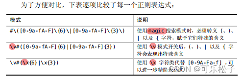
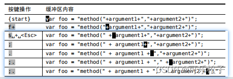
Vim实用技巧_1.vim解决问题的方式
PE format series _0x05: output table and relocation table (.reloc)
深入浅出最优化(2) 步长的计算方法
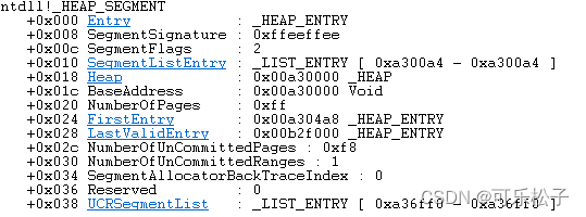
堆(heap)系列_0x03:堆块 + malloc/new底层 + LFH(WinDbg分析)
【深度学习】归一化(十一)
【Likou】1995. Statistical special quadruple
【 graduate work weekly 】 (10 weeks)
Visual Studio 2019新手使用(安装并创建第一个程序详细教程)
人脸识别示例代码解析(一)——程序参数解析
图论最短路径求解
相关性分析
配置 vscode 让它变得更好用
【力扣】516. 最长回文子序列