当前位置:网站首页>Advanced Feature Selection Techniques in Linear Models - Based on R
Advanced Feature Selection Techniques in Linear Models - Based on R
2022-08-10 05:05:00 【Ah Qiangzhen】
Advanced feature selection techniques in linear models——基于R
岭回归
岭回归(英文名:ridge regression, Tikhonov regularization)是一种专用于共线性数据分析的有偏估计回归方法,实质上是一种改良的最小二乘估计法,通过放弃最小二乘法的无偏性,以损失部分信息、降低精度为代价获得回归系数更为符合实际、更可靠的回归方法,对病态数据的拟合要强于最小二乘法.
LASSO
LASSO是由1996年Robert Tibshirani首次提出,全称Least absolute shrinkage and selection operator.该方法是一种压缩估计.它通过构造一个惩罚函数得到一个较为精炼的模型,使得它压缩一些回归系数,即强制系数绝对值之和小于某个固定值;同时设定一些回归系数为零.因此保留了子集收缩的优点,是一种处理具有复共线性数据的有偏估计.
弹性网络
1987Year by Durbin(Durbin)and Will Shaw(Willshaw)在「自然」Resilient Network proposed by the monthly magazine(Elastic Network).这篇只有2页的文章(The Huberfield and Tank papers suffice11页),The first impression is that of intuition,简单,and powerful.A resilient web is a social connection.All your contacts are displayed in the thumbnail list,Sort by the strength of your connection with the person.每当ColorDetects physical proximity between you and another user(i.e. with you),This app will adjust the strength of your relationship.So when you open the app,and when opening your contact list,You'll see close friends and family at the top of the list.
数据理解和准备
The data used in this article is in ElemStatLearn包里面,But for now this package is inrIt cannot be downloaded directly,Here is a method for you
下载方法
以ElemStatLearn包为例
在r studio4.0.3version enteredinstall.packages(“ElemStatLearn”)无法下载ElemStatLearn包
提示CRAN下载地址为https://cran.r-project.org/web/packages/ElemStatLearn/index.html
选择最新版本下载
下载后在r studio中选择Packages——install——install from改为Packages Archive
File(.zip;.tar.gz)——Package archiveSelect the package you just downloaded——点击“Install”安装完成即可library该程序包
library(ElemStatLearn)
prostate

This data was collected97data on ten variables for males,分别为:
- lcavol:Logarithmic tumor volume
- lweight:Logarithm of prostate weight
- age:患者年龄
- lbph:良性前列腺增生(BPH)The logarithmic value of the quantity,Prostate enlargement of a noncancerous nature
- svi:Whether the seminal vesicle has invaded(1代表是,0代表否)
- lcp:The logarithm of the envelope penetration value
- gleason:患者的Gleson评分,The higher the score, the more dangerous it is
- pgg45:Gleson评分为4或5的百分比(High-grade cancer)
- lpsa:PSA值的对数值,响应变量
- train:一个逻辑向量(TRUE or False,Used to distinguish training data from test data)
一. 数据预处理
由于我们的glesonA variable is a characteristic variable,We can turn it into an indicator variable,0Represents a rating of 6,1Indicates a rating of 7或者更高,All you need is this line of code
prostate$gleason <- ifelse(prostate$gleason==6,0,1)
相关系数矩阵:
library(corrplot)
corrplot(cor(prostate))

二.训练集和测试集的划分
train <- subset(prostate,train=T)[,1:9]
test <- subset(prostate,train=F)[,1:9]
prostateThe last column of the dataset is named train,若train=trueis the training set otherwise the test set
We only need to extract the training set and test set from it
三.模型构建与评价
1.最优子集
library(leaps)
a <- regsubsets(lpsa~.,data=train)
b <- summary(a)
which.min(b$bic)
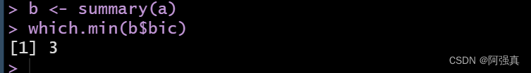
通过BIC信息准则来看,We should choose3an optimal subset
plot(a,scale = "bic",main="Best Sunset Features")

So the above figure tells us that we have the smallestBICvalue in the model3个特征是:lcavol,lweight和svi
Fitting is done below:
ols <- lm(lpsa~lcavol+svi+lweight,data=train)
plot(ols$fitted.values,train$lpsa,xlab="Predicted"
     ,ylab="Acuual",main="Predicted vs Actual")

从图中可以看出,Fits well linearly on the training set,There is also no heteroscedasticity.Then see how the model performs on the test set,使用predicte函数指定newdata=test,如下所示:
pred.test <- predict(ols,newdata=test)
  plot(pred.test,test$lpsa,
       xlab="Predicted"
      ,ylab="Acuual",main="Predicted vs Actual")
Calculate the square of the residuals:
resid <- test$lpsa-pred.test
mean(resid^2)

MSE值为0.488Continue with the following content based on this
2.岭回归
在岭回归中,Our model will cover it all8个特征,The package for using ridge regression isglmnet.Ridge regression requires data to be a matrix rather than a data frame.The command format for ridge regression is glment(x=矩阵,y=响应变量,famliy=分布函数,alpha=0)当alpha=0is to indicate the use of ridge regression,当alpha=1时表示使用LASSO回归
First convert the data to matrix form
x <- as.matrix(train[,1:8])
y <- train[,9]
ridge <- glmnet(x,y,famliy="gaussian",alpha=0)
 print(ridge)

The degrees of freedom can be seen in the first rowdf=7,That is, the number of features included in the model is 7.Remember in ridge regression
,这个数量是不变的.Interpretation bias can also be seen(%DEV)为0.00,and the tuning factor for this linelambda为878,Here you can decide which one to use on which test setlambda.我们首先来看一下,Basic statistical graphs,使用label=TCurves can be annotated
plot(ridge,label=TRUE)

You can see that the abscissa is L1范数,We can also change it to lambda或者dev
plot(ridge,label=TRUE,xvar = "dev")
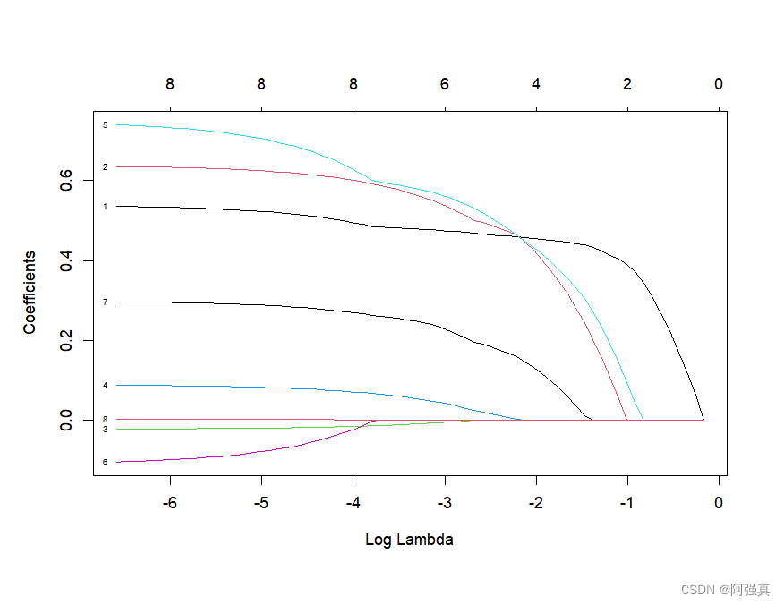
plot(ridge,label=TRUE,xvar="lambda")


This picture is very valuable,它表明当lambda值减少时,The compression parameters are reduced accordingly,The absolute value of the coefficient increases accordingly.要想看lambdafor a specific value is,可以使用coef命令.现在看一下lambda为0.1时,What is the coefficient value.指定参数lambda=0.1,如下所示:
ridge.coef <- coef(ridge,s=0.1)
ridge.coef

需要注意的是pgg45,lcp,ageThe coefficient values are close to 0,但还不是0.Next, let's take a look at the effect on the test set:
newx <- as.matrix(test[,1:8])
length(newx)
ridge.y <- predict(ridge,newx = newx,type="response",s=0.1)
plot(ridge.y,test$lpsa,
     xlab="Predicted"
    ,ylab="Acuual",main="Ridge Regression")
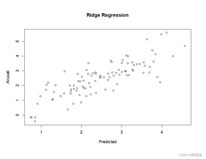
Calculates the mean of the squared residuals:
ridge.resid <- ridge.y-test$lpsa
mean(ridge.resid^2)

相比较于之前的0.48,这里的44A little less,这时候看一下LASSO回归的效果
3.LASSO回归
lasso <- glmnet(x,y,family = "gaussian",alpha=1)
print(lasso)

It can be seen that the first column is the degree of freedom by7变为8时,lambda大约为0.023,So we should use thislambda值
plot(lasso,label=T,xvar="lambda")
lasso.y <- predict(lasso,newx = newx,type="response",s=0.023)
lasso.resid <- lasso.y-test$lpsa
mean(lasso.resid^2)

输出结果为0.44Pretty much the same as Ridge Regression
4.弹性网络
caretThe package is designed to solve classification problems and train regression models.First we need to find the focus onKaTeX parse error: Undefined control sequence: \弹 at position 9: \lambda和\̲弹̲Sex network mixing parametersalpha的最优组合.可以通过下面3completed in one simple step:
- 使用Rin the base packageexpand.grid()函数,Set up a vector to store what we're going to study α 和 λ \alpha和\lambda α和λof all combinations
- 使用caret包中的trainControl()The function determines the resampling method
- P在caret包中的train()函数使用glmnet()Train the model to choose α 和 λ \alpha和\lambda α和λ
Hyperparameters can be selected according to the following two rules - α \alpha α从0到1,每次增加0.2;请记住 α \alpha α被绑定在0到1之间
- λ \lambda λ从0.到0.2,使lassoRegression and Ridge Regression λ \lambda λ位于这个 λ \lambda λ之间
具体操作如下:
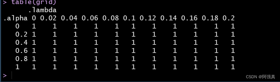
grid <- expand.grid(.alpha=seq(0,1,0.2),.lambda=seq(0.,0.2,0.02))
table(grid)
for resampling methods,We're going to put in the codemethod参数指定为LOOCV.然后通过trainfunction to determine the optimal elastic network.这个函数和lm函数很相似,Just add in the function syntaxmethod=“glmnet”,
trControl=control,tuneGrid=grid.将结果存储在enent.train的对象中
library(caret)
control <- trainControl(method="LOOCV")
enet.train <- train(lpsa~.,data=train,method="glmnet",
                 trControl=control,tuneGrid=grid)
enet.train
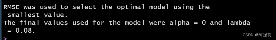
The best results can be seen α = 0 , λ = 0.08 \alpha=0,\lambda=0.08 α=0,λ=0.08
验证模型效果:
enet <- glmnet(x,y,family = "gaussian",alpha=0,lambda=0.08)
coef(enet,s=0.08,exact=T)
enet.y <- predict(enet,newx=newx,type="response",s=0.08)
plot(enet.y,test$lpsa,
xlab="Predicted"
,ylab="Acuual",main="Elastic Net")
mean((enet.y-test$lpsa)^2)
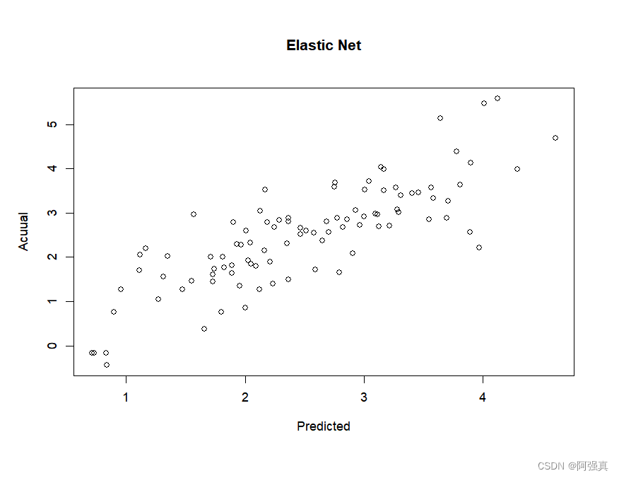


It can be seen that the error is approx0.43Compared with the previous two, it has been improved,So we should choose this method of elastic network
Hence the regression equation is obtained:
l p s a = 0.34 + 0.47 l c a v o l + 0.61 l w e i g h t − 0.01 a g e + 0.07 l b p h + 0.67 s v i − 0.04 l c p + 0.29 g l e s o n + 0.002 p g g 45 lpsa=0.34+0.47lcavol+0.61lweight-0.01age+0.07lbph+\\ 0.67svi-0.04lcp+0.29gleson+0.002pgg45 lpsa=0.34+0.47lcavol+0.61lweight−0.01age+0.07lbph+0.67svi−0.04lcp+0.29gleson+0.002pgg45
边栏推荐
猜你喜欢

小影科技IPO被终止:年营收3.85亿 五岳与达晨是股东

线程(下):读写者模型\环形队列\线程池

【u-boot】u-boot驱动模型分析(02)

leetcode每天5题-Day12

How to choose the right oscilloscope probe in different scenarios

webrtc学习--websocket服务器(二) (web端播放h264)
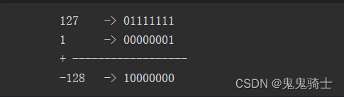
Why are negative numbers in binary represented in two's complement form - binary addition and subtraction
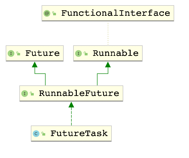
60行从零开始自己动手写FutureTask是什么体验?

顺序表的删除,插入和查找操作

线程(中):线程安全
随机推荐
Rpc接口压测
Acwing 59. 把数字翻译成字符串 计数类DP
Order table delete, insert and search operations
aliases节点分析
SQL Server查询优化
解决“File has been changed outside the editor, reload?”提示
2022年T电梯修理考试题及模拟考试
Unity Shader 积雪效果
【论文笔记】Prototypical Contrast Adaptation for Domain Adaptive Semantic Segmentation
深度学习之-01
Shell编程三剑客之awk
成为黑客不得不学的语言,看完觉得你们还可吗?
二进制中负数为何要用补码形式来表示——二进制加减法
How to choose the right oscilloscope probe in different scenarios
Ask you guys.The FlinkCDC2.2.0 version in the CDC community has a description of the supported sqlserver version, please
华为交换机配置日志推送
FPGA工程师面试试题集锦21~30
干货 | 查资料利器:线上图书馆
canvas 画布绘制时钟
元宇宙 | 你能通过图灵测试吗?