项目2-Annual income judgment

友情提示

Students can go to the course work area to try it out first！！！

项目描述

二元分类是机器学习中最基础的问题之一,在这份教学中,你将学会如何实作一个线性二元分类器,来根据人们的个人资料,判断其年收入是否高于 50,000 美元.我们将以两种方法: logistic regression 与 generative model,来达成以上目的,你可以尝试了解、分析两者的设计理念及差别.
实现二分类任务：

• 个人收入是否超过50000元？

数据集介绍

这个资料集是由UCI Machine Learning Repository 的Census-Income (KDD) Data Set 经过一些处理而得来.为了方便训练,We removed some unnecessary information,And slightly balance the ratio of positive and negative markers.事实上在训练过程中,只有 X_train、Y_train 和 X_test 这三个经过处理的档案会被使用到,train.csv 和 test.csv 这两个原始资料档则可以提供你一些额外的资讯.

• Unnecessary attributes have been removed.
• The ratio between positive and negative scaled data has been balanced.

特征格式

1. train.csv,test_no_label.csv.

• Text-based raw data
• 去掉不必要的属性,Balance positive and negative ratios.

2. X_train, Y_train, X_test(测试)

• train.csvdiscrete features in =>在X_train中onehot编码(学历、martial arts status…)
• train.csvcontinuous features in => 在X_train中保持不变(年龄、资本损失…).
• X_train, X_test : 每一行包含一个510-dim的特征,代表一个样本.
• Y_train: label = 0 表示 “<=50K” 、 label = 1 表示 " >50K " .

项目要求

1. Please write it yourself gradient descent 实现 logistic regression
2. Get your hands on a probabilistic generative model.
3. A single block of code should run for less than five minutes.
4. The use of any open source code is prohibited(例如,你在GitHubAn implementation of the decision tree found on ).

数据准备

项目数据保存在：work/data/ 目录下.

环境配置/安装

无

Logistic回归

First we will do it Logistic回归

数据准备

下载资料,And normalize each attribute,After processing, it is divided into training set and validation set.

import numpy as np
import pandas as pd

X_train_fpath = 'work/data/X_train'
with open(X_train_fpath) as f:
    X_train = np.array([line.strip('\n').split(',')[1:] for line in f])
    print(X_train)
    X_train = pd.DataFrame(X_train[1:],index=None,columns = X_train[0])
    print(X_train.head())
print(X_train.shape)

[['age' ' Private' ' Self-employed-incorporated' ...
  'weeks worked in year' ' 94' ' 95']
 ['33' '1' '0' ... ' 52' '0' '1']
 ['63' '1' '0' ... ' 52' '0' '1']
 ...
 ['16' '0' '0' ... ' 8' '1' '0']
 ['48' '1' '0' ... ' 52' '0' '1']
 ['48' '0' '0' ... ' 0' '0' '1']]
 
 
  age  Private  Self-employed-incorporated  State government  ...
0  33        1                           0                 0   
1  63        1                           0                 0   
2  71        0                           0                 0   
3  43        0                           0                 0   
4  57        0                           0                 0   
[5 rows x 510 columns]


(54256, 510)

import numpy as np

np.random.seed(0)
X_train_fpath = 'work/data/X_train'
Y_train_fpath = 'work/data/Y_train'
X_test_fpath = 'work/data/X_test'
output_fpath = 'work/output_{}.csv'

# 将CSV文件解析为NumPy数组
with open(X_train_fpath) as f:
    next(f)
    X_train = np.array([line.strip('\n').split(',')[1:] for line in f], dtype = float)
with open(Y_train_fpath) as f:
    next(f)
    Y_train = np.array([line.strip('\n').split(',')[1] for line in f], dtype = float)
with open(X_test_fpath) as f:
    next(f)
    X_test = np.array([line.strip('\n').split(',')[1:] for line in f], dtype = float)

def _normalize(X, train = True, specified_column = None, X_mean = None, X_std = None):
    # This function is used for normalizationX的特定列.
    # when processing test data,The mean and standard deviation of the training data will be reused.
    # 参数：
    # X：待处理数据.
    # Train：When processing training data‘True’,When processing test data‘False.
    # SPECIAL_COLUMN：The index of the column that will be normalized.如果为‘None’,then all columns.
    # 归一化.
    # X_Mean：The mean of the training data,当Train=‘False’时使用.
    # X_STD：The standard deviation of the training data,当Train=‘False’时使用.
    # 输出：
    # X：归一化数据.
    # X_Mean：The computed mean of the training data.
    # X_STD：The computed standard deviation of the training data

    if specified_column == None:
        specified_column = np.arange(X.shape[1])
    if train:
        X_mean = np.mean(X[:, specified_column] ,0).reshape(1, -1)
        X_std  = np.std(X[:, specified_column], 0).reshape(1, -1)

    X[:,specified_column] = (X[:, specified_column] - X_mean) / (X_std + 1e-8)
     
    return X, X_mean, X_std

def _train_dev_split(X, Y, dev_ratio = 0.25):
    # This function splits the data into training and validation sets,dev_ratioRepresents the proportion of the validation set
    train_size = int(len(X) * (1 - dev_ratio))
    return X[:train_size], Y[:train_size], X[train_size:], Y[train_size:]

# Normalize training and test data
X_train, X_mean, X_std = _normalize(X_train, train = True)
X_test, _, _= _normalize(X_test, train = False, specified_column = None, X_mean = X_mean, X_std = X_std)
    
# Split the data into training and validation sets
dev_ratio = 0.1
X_train, Y_train, X_dev, Y_dev = _train_dev_split(X_train, Y_train, dev_ratio = dev_ratio)

train_size = X_train.shape[0]
dev_size = X_dev.shape[0]
test_size = X_test.shape[0]
data_dim = X_train.shape[1]
print('Size of training set: {}'.format(train_size))
print('Size of validation set: {}'.format(dev_size))
print('Size of testing set: {}'.format(test_size))
print('Dimension of data: {}'.format(data_dim))

Size of training set: 48830
Size of validation set: 5426
Size of testing set: 27622
Dimension of data: 510

一些有用的函数

These functions may be used repeatedly in the training loop.

def _shuffle(X, Y):
    # This function takes two lists of equal length/数组X和Ymess up together
    randomize = np.arange(len(X))
    np.random.shuffle(randomize)
    return (X[randomize], Y[randomize])

def _sigmoid(z):
    # SigmoidFunctions can be used to calculate probabilities.
    # 为了避免溢出,The minimum output value is set1e-8,maximum output value1 - (1e-8).
    return np.clip(1 / (1.0 + np.exp(-z)), 1e-8, 1 - (1e-8))

def _f(X, w, b):
    # This is the logistic regression function,参数为w和b
    # 参数:
    # X: input data, shape = [batch_size, data_dimension]
    # w: 权重向量,形状= [data_dimension,]
    # b: 偏置值,标量
    # 输出:
    # np.matmul返回两个数组的矩阵乘积：z=x*w+b
    # X：The predicted probability that each row is positively marked,shape = [batch_size,]
    return _sigmoid(np.matmul(X, w) + b)

def _predict(X, w, b):
    # 这个函数返回XThe ground truth prediction for each row
    # By rounding the result of the logistic regression function.
    return np.round(_f(X, w, b)).astype(np.int)
    
def _accuracy(Y_pred, Y_label):
    # This function calculates the prediction accuracy
    # np.abs求绝对值
    acc = 1 - np.mean(np.abs(Y_pred - Y_label))
    return acc

Gradient and loss

def _cross_entropy_loss(y_pred, Y_label):
    # This function calculates cross entropy.
    # 输入:
    # y_pred: 概率预测,浮点向量
    # Y_label: 真实标签,bool向量
    # 输出:
    # np.dotThe role is vector dot product and matrix multiplication
    # logIf nothing is written, the default is to find the natural logarithm
    # cross_entropy：交叉熵,标量,cross_entropy = y真*lny预 - (1-y真)*ln(1-y预)
    cross_entropy = -np.dot(Y_label, np.log(y_pred)) - np.dot((1 - Y_label), np.log(1 - y_pred))
    return cross_entropy

def _gradient(X, Y_label, w, b):
    # This function calculates relative weightsw和偏置值bThe cross-entropy loss gradient of 
    # np.sum中,当axis为0时,是压缩行,即将每一列的元素相加,将矩阵压缩为一行
    # 当axis为1时,是压缩列,即将每一行的元素相加,将矩阵压缩为一列
    y_pred = _f(X, w, b)
    pred_error = Y_label - y_pred
    w_grad = -np.sum(pred_error * X.T, 1)
    b_grad = -np.sum(pred_error)
    return w_grad, b_grad

模型训练

一切准备就绪,开始训练吧!

We use mini-batch gradient descent for training.The training data is divided into many small batches,针对每一个小批次,我们分别计算其梯度以及损失,并根据该批次来更新模型的参数.When a loop is completed,也就是整个训练集的所有小批次都被使用过一次以后,We shred all training data and re-split into new mini-batches,Take the next loop,until the preset number of laps is reached.

# Zero initialization of weights and biases
# np.zeros((data_dim,))：to get a full row0的列表,个数为：data_dim
w = np.zeros((data_dim,)) 
b = np.zeros((1,))

# Some parameters for training
max_iter = 10
batch_size = 8
learning_rate = 0.2

# Maintains loss and precision for each iteration,进行绘图
train_loss = []
dev_loss = []
train_acc = []
dev_acc = []

# Counts the number of parameter updates
step = 1

# 迭代训练
for epoch in range(max_iter):
    # The training set is randomly shuffled in each round of iterationsX_train和验证集Y_train
    X_train, Y_train = _shuffle(X_train, Y_train)
        
    # 小批次训练,Used to return the lower bound of the input element-wise.
    for idx in range(int(np.floor(train_size / batch_size))):
        X = X_train[idx*batch_size:(idx+1)*batch_size]
        Y = Y_train[idx*batch_size:(idx+1)*batch_size]

        # 计算梯度
        w_grad, b_grad = _gradient(X, Y, w, b)
            
        # 梯度下降更新
        # 学习率随时间衰减
        w = w - learning_rate/np.sqrt(step) * w_grad
        b = b - learning_rate/np.sqrt(step) * b_grad

        step = step + 1
            
    # Calculate loss and accuracy on training and validation sets
    y_train_pred = _f(X_train, w, b)
    Y_train_pred = np.round(y_train_pred)
    train_acc.append(_accuracy(Y_train_pred, Y_train))
    train_loss.append(_cross_entropy_loss(y_train_pred, Y_train) / train_size)

    y_dev_pred = _f(X_dev, w, b)
    Y_dev_pred = np.round(y_dev_pred)
    dev_acc.append(_accuracy(Y_dev_pred, Y_dev))
    dev_loss.append(_cross_entropy_loss(y_dev_pred, Y_dev) / dev_size)

print('Training loss: {}'.format(train_loss[-1]))
print('validation loss: {}'.format(dev_loss[-1]))
print('Training accuracy: {}'.format(train_acc[-1]))
print('validation accuracy: {}'.format(dev_acc[-1]))

Training loss: 0.271355435246406
validation loss: 0.28963596750262866
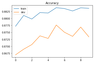
Training accuracy: 0.8836166291214418
validation accuracy: 0.8733873940287504

Plot loss and accuracy curves

%matplotlib inline
import matplotlib.pyplot as plt

# 损失曲线
plt.plot(train_loss)
plt.plot(dev_loss)
plt.title('Loss')
plt.legend(['train', 'dev'])
plt.savefig('loss.png')
plt.show()

# 精度曲线
plt.plot(train_acc)
plt.plot(dev_acc)
plt.title('Accuracy')
plt.legend(['train', 'dev'])
plt.savefig('acc.png')
plt.show()

Predict test labels

The data labels for the test set are predicted and exist output_logistic.csv 中.

# 预测测试集标签
predictions = _predict(X_test, w, b)
with open(output_fpath.format('logistic'), 'w') as f:
    f.write('id,label\n')
    for i, label in enumerate(predictions):
        f.write('{},{}\n'.format(i, label))

# Print out the most important ones10个权重w
# np.argsortReturns an array of index values ​​sorted from smallest to largest
# [::-1]将数组倒序
ind = np.argsort(np.abs(w))[::-1]
with open(X_test_fpath) as f:
    content = f.readline().strip('\n').split(',')
features = np.array(content)
for i in ind[0:10]:
    print(features[i], w[i])

 Not in universe -4.031960278019252
 Spouse of householder -1.6254039587051405
 Other Rel <18 never married RP of subfamily -1.4195759775765409
 Child 18+ ever marr Not in a subfamily -1.2958572076664745
 Unemployed full-time 1.1712558285885908
 Other Rel <18 ever marr RP of subfamily -1.1677918072962366
 Italy -1.0934581438006177
 Vietnam -1.0630365633146412
num persons worked for employer 0.9389922773566517
 1 0.822661492211719

Multivariate generative models

Then we will implement the base generative model 的二元分类器.

数据准备

训练集与测试集的处理方法跟 logistic regression 一模一样,然而因为 generative model 有可解析的最佳解,因此不必使用到验证集.

# 将CSV文件解析为NumPy数组
with open(X_train_fpath) as f:
    next(f)
    X_train = np.array([line.strip('\n').split(',')[1:] for line in f], dtype = float)
with open(Y_train_fpath) as f:
    next(f)
    Y_train = np.array([line.strip('\n').split(',')[1] for line in f], dtype = float)
with open(X_test_fpath) as f:
    next(f)
    X_test = np.array([line.strip('\n').split(',')[1:] for line in f], dtype = float)

# 归一化
X_train, X_mean, X_std = _normalize(X_train, train = True)
X_test, _, _= _normalize(X_test, train = False, specified_column = None, X_mean = X_mean, X_std = X_std)

mean and covariance

在 generative model 中,We need to calculate the mean and covariation of the data within the two categories separately.

# Calculate the within-class mean
X_train_0 = np.array([x for x, y in zip(X_train, Y_train) if y == 0])
X_train_1 = np.array([x for x, y in zip(X_train, Y_train) if y == 1])

mean_0 = np.mean(X_train_0, axis = 0)
mean_1 = np.mean(X_train_1, axis = 0)  

# 计算类内协方差
cov_0 = np.zeros((data_dim, data_dim))
cov_1 = np.zeros((data_dim, data_dim))

for x in X_train_0:
    cov_0 += np.dot(np.transpose([x - mean_0]), [x - mean_0]) / X_train_0.shape[0]
for x in X_train_1:
    cov_1 += np.dot(np.transpose([x - mean_1]), [x - mean_1]) / X_train_1.shape[0]

# The shared covariance is the weighted average of the individual within-class covariances.
cov = (cov_0 * X_train_0.shape[0] + cov_1 * X_train_1.shape[0]) / (X_train_0.shape[0] + X_train_1.shape[0])

计算权重和偏差

权重矩阵与偏差向量可以直接被计算出来.

# 计算协方差矩阵的逆矩阵.
# Since the covariance matrix may be nearly singular,np.linalg.inv()May give large numerical errors.
# 通过SVD分解,The inverse of a matrix can be obtained efficiently and accurately.
u, s, v = np.linalg.svd(cov, full_matrices=False)
inv = np.matmul(v.T * 1 / s, u.T)

# Calculate the weights directlyw和偏差b
w = np.dot(inv, mean_0 - mean_1)
b =  (-0.5) * np.dot(mean_0, np.dot(inv, mean_0)) + 0.5 * np.dot(mean_1, np.dot(inv, mean_1))\
    + np.log(float(X_train_0.shape[0]) / X_train_1.shape[0]) 

# Calculate the accuracy on the training set
Y_train_pred = 1 - _predict(X_train, w, b)
print('Training accuracy: {}'.format(_accuracy(Y_train_pred, Y_train)))

Training accuracy: 0.8671114715423179

Predict test labels

The data labels for the test set are predicted and exist output_generative.csv 中.

# 预测测试集标签
predictions = 1 - _predict(X_test, w, b)
with open(output_fpath.format('generative'), 'w') as f:
    f.write('id,label\n')
    for i, label in  enumerate(predictions):
        f.write('{},{}\n'.format(i, label))

# Print out the most important ones10个权重w
ind = np.argsort(np.abs(w))[::-1]
with open(X_test_fpath) as f:
    content = f.readline().strip('\n').split(',')
features = np.array(content)
for i in ind[0:10]:
    print(features[i], w[i])

 Retail trade 7.67333984375
 Midwest -6.3125
 34 -5.835205078125
 37 -5.489013671875
 Child <18 ever marr not in subfamily -5.4759521484375
 Other service -5.00390625
 Different county same state 4.66796875
 33 -3.91015625
 Private household services 3.8623046875
 32 -3.51953125