损失函数——交叉熵

在了解交叉熵之前我们需要关于熵的一些基本知识，可以参考我的上一篇博客¹。

1.信息熵

信息熵的定义为离散随机事件的出现概率²。当一个事件出现的概率更高的时候，我们认为该事件会传播的更广，因此可以使用信息熵来衡量信息的价值。
当一个信源具有多种不同的结果，记为：U1,U2,…,Un，每个事件相互独立，对应的概率记为:P1,P2,…,Pn。信息熵为各个事件方式概率的期望，公式为：
$$H(U)=E[-\log p_i]=-\sum _{i=1}^n{p}_i\log p_i$$

对于二分类问题，当一种事件发生的概率为p时，另一种事件发生的概率就为(1-p)，因此，对于二分类问题的信息熵计算公式为：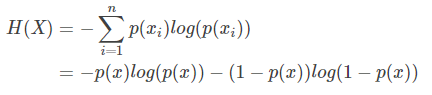

2.相对熵(KL散度)

相对熵(relative entropy)，又被称为Kullback-Leibler散度(Kullback-leibler divergence)，是两个概率分布间差异的一种度量³。在信息论中，相对熵等于两个概率分布的信息熵的差值。
相对熵的计算公式为：
KaTeX parse error: No such environment: align at position 8: \begin{̲a̲l̲i̲g̲n̲}̲ \text{KL}(P||Q…
其中$p(x)$代表事件的真实概率，$q(x)$代表事件的预测概率。例如三分类问题的标签为$(1,0,0)$，预测标签为$(0.7,0.1,0.2)$。

因此该公式的字面上含义就是真实事件的信息熵与理论拟合的事件的香农信息量与真实事件的概率的乘积的差的累加。[4]

当p(x)和q(x)相等时相对熵为0，其它情况下大于0。证明如下：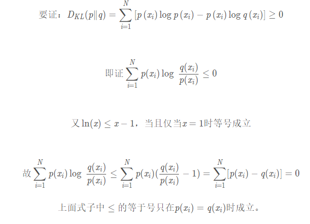

KL散度在Pytorch中的使用方法为：

torch.nn.KLDivLoss(size_average=None, reduce=None, reduction='mean', log_target=False)

在使用过程中，reduction一般设置为batchmean这样才符合数学公式而不是mean，在以后的版本中mean会被替换掉。
此外，还要注意log_target参数，因为在计算的过程中我们往往使用的是log softmax函数而不是softmax函数来避免underflow和overflow问题，因此我们要提前了解target是否经过了log运算。

torch.nn.KLDivLoss()会传入两个参数(input, target), input是模型的预测输出，target是样本的观测标签。

kl_loss = nn.KLDivLoss(reduction="batchmean")
output = kl_loss(input, target)

下面我们用一个例子来看看torch.nn.KLDivLoss()是如何使用的：

import torch
import torch.nn as nn
import torch.nn.functional as F

input = torch.randn(3, 5, requires_grad=True)
input = F.log_softmax(input, dim=1)  # dim=1 每一行为一个样本

target = torch.rand(3,5)

# target使用softmax
kl_loss = nn.KLDivLoss(reduction="batchmean", log_target=False)
output = kl_loss(input, F.softmax(target, dim=1))
print(output)

# target使用log_softmax
kl_loss_log = nn.KLDivLoss(reduction="batchmean", log_target=True)
output = kl_loss_log(input, F.log_softmax(target, dim=1))
print(output)

输出结果如下：

tensor(0.3026, grad_fn=<DivBackward0>)
tensor(0.3026, grad_fn=<DivBackward0>)

3.交叉熵

相对熵可以写成如下形式：
$$D_{KL}(p||q)=\sum _{i=1}^{n}p(x_i)\log p(x_i)-\sum _{i=1}^{n}p(x_i)\log q(x_i)=-H(p(x))+[-\sum _{i=1}^{n}p(x_i)\log q(x_i)]$$
等式的前一项为真实事件的熵，后一部分为交叉熵⁴：
$$H（p,q）=-\sum _{i=1}^{n}p(x_i)\log q(x_i)$$
在机器学习中，使用KL散度就可以评价真实标签与预测标签间的差异，但由于KL散度的第一项是个定值，故在优化过程中只关注交叉熵就可以了。一般大多数机器学习算法会选择交叉熵作为损失函数。

交叉熵在pytorch中可以调用如下函数实现：

torch.nn.CrossEntropyLoss(weight=None, size_average=None, ignore_index=-100, reduce=None, reduction='mean')

其计算方法如下所示⁵：
假设batch size为4，待分类标签有3个，隐藏层的输出为：

input = torch.tensor([[ 0.8082,  1.3686, -0.6107],
                      [ 1.2787,  0.1579,  0.6178],
                      [-0.6033, -1.1306,  0.0672],
                      [-0.7814,  0.1185, -0.2945]])

经过softmax激活函数之后得到预测值：

output = nn.Softmax(dim=1)(input)

output:
tensor([[0.3341, 0.5851, 0.0808],
        [0.5428, 0.1770, 0.2803],
        [0.2821, 0.1665, 0.5515],
        [0.1966, 0.4835, 0.3199]])

softmax函数的输出结果每一行相加为1。
假设这一个mini batch的标签为

[1,0,2,1]

根据交叉熵的公式：
$$H（p,q）=-\sum _{i=1}^{n}p(x_i)\log q(x_i)$$
$p(x_i)$代表真实标签，在真实标签中，除了对应类别其它类别的概率都为0，实际上，交叉熵可以简写为：
$H(p,q)=-\log q(x_{class})$
所以该mini batch的loss的计算公式为（别忘了除以batch size，我们最后求得的是mini batch的平均loss）：
$Loss=-[log(0.5851)+log(0.5428)+log(0.5515)+log(0.4835)]/4$
因此，我们还需要计算一次对数：

output_log = torch.log(output)
output_log

计算结果为：

tensor([[-1.0964, -0.5360, -2.5153],
        [-0.6111, -1.7319, -1.2720],
        [-1.2657, -1.7930, -0.5952],
        [-1.6266, -0.7267, -1.1397]])

根据交叉熵的计算公式，loss的最终计算等式为：
$loss=-(-0.5360-0.6111-0.5952-0.7267)/4=0.61725$
运算结果和pytorch内置的交叉熵函数相同：

import torch
import torch.nn as nn

input = torch.tensor([[ 0.8082,  1.3686, -0.6107],
        [ 1.2787,  0.1579,  0.6178],
        [-0.6033, -1.1306,  0.0672],
        [-0.7814,  0.1185, -0.2945]])
target = torch.tensor([1,0,2,1])

loss = nn.CrossEntropyLoss()
output = loss(input, target)
output.backward()

结果为：

tensor(0.6172)

除了torch.nn.CrosEntropyLoss()函数外还有一个计算交叉熵的函数torch.nn.BCELoss()。与前者不同，该函数是用来计算二项分布（0-1分布）的交叉熵，因此输出层只有一个神经元（只能输出0或者1）。其公式为：
$$loss=-[y\cdot logx+(1-y)\cdot log(1-x)]$$
在pytorch中的函数为：

torch.nn.BCELoss(weight=None, size_average=None, reduce=None, reduction='mean')

用一个实例来看看如何使用该函数：

input = torch.tensor([-0.7001, -0.7231, -0.2049])
target = torch.tensor([0,0,1]).float()
m = nn.Sigmoid()
loss = nn.BCELoss()
output = loss(m(input), target)
output.backward()

输出结果为：

tensor([0.5332])

它是如何计算的呢，我们接下来一步步分析：

首先输入是:

input = [-0.7001, -0.7231, -0.2049]

需要经过sigmoid函数得到一个输出

output_mid = m(input)

输出结果为：

[0.3318, 0.3267, 0.4490]

然后我们根据二项分布交叉熵的公式：
$$loss=-[y\cdot logx+(1-y)\cdot log(1-x)]$$
得到loss的如下计算公式：

$loss=-[1\ast \log (1-0.3318)+1\ast \log (1-0.3267)+1\ast \log (0.4490)]/3=0.5312$

和pytorch的内置函数计算结果相同。