分割画布函数详解

一.前言

在使用matplotlib库进行数据可视化的过程中，我们都离不开一个重要载体–画布（Figure）。一个Figure对象是所有绘图元素的顶层容器，想要实现画布的合理使用，分区使用必不可少。

---

首先理解一下子区这个概念，子区顾名思义就是将大画布（FIgure）划分成若干个子画布，这些子画布构成绘图区域，其本质是在纵横交错的行列网格中添加坐标轴系统。接下来主要介绍一下3个相关函数，下文中的所有实例代码均在Ipython上实现，且相关库导入以及中文修改语句已经省略，文中所提及的方法二字和函数等价。

---

二.subplots函数

这个函数最为简单直接，调用plt.subplots()会直接创建一个1行1列的网格布局子区间，同时创建一个Figure对象。

2.1函数定义

subplots(nrows=1, 
		ncols=1, 
		*, 
		sharex=False,
		sharey=False, 
		squeeze=True, 
		subplot_kw=None, 
		gridspec_kw=None, 
		fig_kw)

参数说明：

参数1：nrows：整数型，指定子图网格的行数

参数2：ncols：整数型，指定子图网格的列数

参数3：sharex：布尔型或字符型，指定是否共享x轴，可选{‘none’，‘all’，‘row’，‘col’}

​ none：等同于False，指定所有子图不共享

​ all：指定x轴或y轴将在所有子图之间共享

​ row：指定每行子图将共享一个x轴或y轴

​ col：指定每列子图将共享一个x轴或y轴

参数4：sharey：布尔型或字符型，指定是否共享y轴，可选{‘none’，‘all’，‘row’，‘col’}

​ none：等同于False，指定所有子图不共享

​ all：指定x轴或y轴将在所有子图之间共享

​ row：指定每行子图将共享一个x轴或y轴

​ col：指定每列子图将共享一个x轴或y轴

参数5：squeeze：布尔型，指定是否进行压缩

参数6：subplot_kw：字典型，传递给add_subplot方法，指定创建每个子图的调用的关键字参数

参数7：gridspec_kw：字典型，传递给GridSpec类，指定子图放置的网格的关键字参数

参数8：**fig_kw：字典型，传递给 pyplot.figure方法

返回值1：FIgure实例

返回值2：Axes实例或者Axes实例数组，该数组和网格有相同的形状

---

参数详解：

1. fig_kw的参数传递给pyplot.figure方法的意思是该参数的所有内容会直接传递给plt.figure方法。subplot_kw、subplot_kw同理。
2. 对参数squeeze，如果为True且仅构造一个子图，则返回的单个Axes对象将作为标量返回。对于Nx1或1xM子图，返回的对象是包含Axes对象的numpy数组。对于N×M个，副区与N> 1和M> 1返回为2D阵列。如果为False，则完全不进行压缩：返回的Axes对象始终是包含Axes实例的2D数组，即使最终它是1x1。具体示例见下文。

---

2.2函数讲解

这个函数的优势是一步到位，创建Figure对象的同时创建指定行列的网格布局，在代码量上减少了很多。下文是该函数的内部实现：

fig = figure(fig_kw)	#创建Figure对象
axs = fig.subplots(nrows=nrows, 	#指定行
					ncols=ncols, 	#指定列
					sharex=sharex, 	#指定是否共享X轴
					sharey=sharey,	#指定是否共享y轴
                    squeeze=squeeze, 	#指定是否进行返回值压缩
                    subplot_kw=subplot_kw,	
                    gridspec_kw=gridspec_kw)
return fig, axs	#返回Figure对象和坐标轴系统

可以看到调用plt.figure函数并传递参数fig_kw并创建一个Figure对象，这就是上文中说传递给plt.figure函数的意思。接着调用Figure.subplots方法创建网格布局和坐标轴系统。下文是fig.subplots的核心代码：

  if self.get_constrained_layout():
  		gs = GridSpec(nrows, ncols, figure=self, gridspec_kw)	#创建GridSpec类实例
  else:
        # this should turn constrained_layout off if we don't want it
        gs = GridSpec(nrows, ncols, figure=None, gridspec_kw)
  self._gridspecs.append(gs)

  # Create array to hold all axes.
  axarr = np.empty((nrows, ncols), dtype=object)	#创建一个空矩阵，类型是对象
  #循环创建坐标轴系统，下标0开始
  for row in range(nrows):
  		for col in range(ncols):
        	shared_with = {
    "none": None, "all": axarr[0, 0],"row": axarr[row, 0], "col": axarr[0, col]}	#sharex和sharey的检查字典
            subplot_kw["sharex"] = shared_with[sharex]	#字典取值
            subplot_kw["sharey"] = shared_with[sharey]	#字典取值
            axarr[row, col] = self.add_subplot(gs[row, col], subplot_kw)	#创建坐标轴系统
# turn off redundant tick labeling
	#设置共享X轴
  if sharex in ["col", "all"]:
    # turn off all but the bottom row
  	for ax in axarr[:-1, :].flat:
    	ax.xaxis.set_tick_params(which='both', labelbottom=False, labeltop=False)
        ax.xaxis.offsetText.set_visible(False)
  #设置共享Y轴
  if sharey in ["row", "all"]:
  	# turn off all but the first column
    for ax in axarr[:, 1:].flat:
    	ax.yaxis.set_tick_params(which='both', labelleft=False, labelright=False)
        ax.yaxis.offsetText.set_visible(False)
        
  if squeeze:
  		return axarr.item() if axarr.size == 1 else axarr.squeeze()	#调用squeeze方法压删除一维
  else:
        return axarr	#返回一个二维矩阵

首先创建GridSpec类实例，该类用于指定网格的几何形状。然后循环创建坐标轴系统，并添加到一个空矩阵中，此时squeeze参数并产生作用，返回值是一个指定形状的二维矩阵，接下来两个if-for代码块用来设置sharex和sharey参数响应。最后对squeeze参数进行检测，假设为True则依据行列数返回一个纯实例还是二维矩阵，假设为False则无论如何都返回一个二维矩阵。

---

2.3函数示例

2.3.1squeeze参数示例

首先创建一个1行1列的网格布局，squeeze参数为False，看看其返回值：

fig, ax = plt.subplots(squeeze=False)
ax.shape, ax

其结果如下：

((1, 1), array([[<AxesSubplot:>]], dtype=object))

证明返回的是一个二位数组，而不是一个对象，接下来将squeeze参数改为True：

fig, ax = plt.subplots(squeeze=True)
ax

其结果如下：

<AxesSubplot:>

返回值是单纯的一个对象。但是假设我们设定多行或者多列会怎么样呢？

fig, ax2 = plt.subplots(2, 2, squeeze=True)
ax2.shape, ax2

fig, ax1 = plt.subplots(2, 2, squeeze=False)
ax1.shape, ax1

其结果如下：

((2, 2),
 array([[<AxesSubplot:>, <AxesSubplot:>],
        [<AxesSubplot:>, <AxesSubplot:>]], dtype=object))
        
((2, 2),
 array([[<AxesSubplot:>, <AxesSubplot:>],
        [<AxesSubplot:>, <AxesSubplot:>]], dtype=object))        

证明在多行多列的情况下，squeeze是没有影响的。

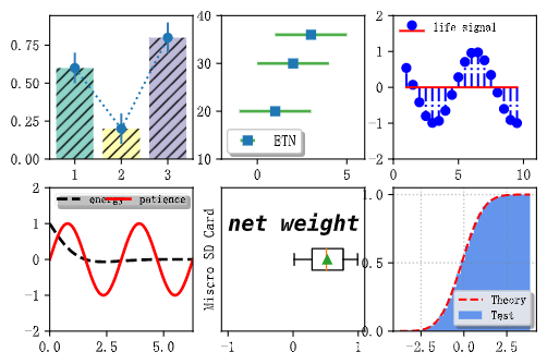
2.3.2综合示例

fig, ax = plt.subplots(2, 3)

colors_list = ['#8dd3c7', '#ffffb3', '#bebada']
ax[0, 0].bar([1, 2, 3], [0.6, 0.2, 0.8], color=colors_list, width=0.8, hatch='///', align='center')
ax[0, 0].errorbar([1, 2, 3], [0.6, 0.2, 0.8], yerr=0.1, capsize=0, ecolor='#377eb8', fmt='o:')

ax[0, 1].errorbar([1, 2, 3], [20, 30, 36], xerr=2, ecolor='#4daf4a', elinewidth=2, fmt='s', label='ETN')
ax[0, 1].legend(loc=3, fancybox=True, shadow=True, fontsize=10, borderaxespad=0.4)
ax[0, 1].set_ylim(10, 40)
ax[0, 1].set_xlim(-2, 6)

x3 = np.arange(1, 10, 0.5)
y3 = np.cos(x3) 

ax[0, 2].stem(x3, y3, basefmt='r-', linefmt='b-.', markerfmt='bo', label='life signal')
ax[0, 2].legend(loc=2, fancybox=True, shadow=True, frameon=False, fontsize=8, borderaxespad=0.6, borderpad=0.0)
ax[0, 2].set_ylim(-2, 2)
ax[0, 2].set_xlim(0, 11)

x4 = np.linspace(0, 2*np.pi, 500)
x4_1 = np.linspace(0, 2*np.pi, 1000)
y4 = np.cos(x4)*np.exp(-x4)
y4_1 = np.sin(2*x4_1)
line1, line2 = ax[1, 0].plot(x4, y4, 'k--', x4_1, y4_1, 'r-', lw=2)
ax[1, 0].legend((line1, line2), ('energy', 'patience'), loc=2, fancybox=True, shadow=True, framealpha=0.3,mode='expand', fontsize=8, ncol=2, columnspacing=2, borderpad=0.1, markerscale=0.1)
ax[1, 0].set_ylim(-2, 2)
ax[1, 0].set_xlim(0, 2*np.pi)

x5 = np.random.rand(100)
ax[1, 1].boxplot(x5, vert=False, showmeans=True, meanprops=dict(color='black'))
ax[1, 1].set_yticks([])
ax[1, 1].set_xlim(-1.1, 1.1)
ax[1, 1].set_ylabel('Miscro SD Card')
ax[1, 1].text(-1.0, 1.2, 'net weight', fontsize=15, style='italic', weight='black', family='monospace')

mu = 0.0
sigma = 1.0

x6 = np.random.randn(10000)
n, bins, patches = ax[1, 2].hist(x6, bins=30, histtype='stepfilled', cumulative=True, color='cornflowerblue', 
label='Test', density=True)
y = ((1 / (np.sqrt(2 * np.pi) * sigma)) * np.exp(-0.5 * (1 / sigma * (bins-mu))  2))
y = y.cumsum()
y /= y[-1]

ax[1, 2].plot(bins, y, 'r--', lw=1.5, label='Theory')
ax[1, 2].set_ylim([0.0, 1.1])
ax[1, 2].grid(ls=':', lw=1, color='grey', alpha=0.5)
ax[1, 2].legend(fontsize=8, shadow=True, fancybox=True, framealpha=0.8)
ax[1, 2].autoscale()

plt.show()

其结果如下：

---

三.plt.subplot函数

该函数是一个对Figure.add_subplot方法的包装，他的作用在于将轴添加到现有Figure对象，或者检索现有轴，其核心语句就是fig = gcf()获取当前Figure对象。

3.1函数定义

subplot有多种形式，其部分示例如下：

subplot(nrows, ncols, index, kwargs)
subplot(pos, kwargs)
subplot(kwargs)
subplot(ax)

参数说明：

参数1：* args：指定描述子图的方法

​ （nrows，ncols，index）：指定行数、列数和当前激活子图索引，索引从左上角的1开始并向右增加。索引也可以是两元素元组指定（start， end） ，即绘制一个跨区子图

​ 三位整数：百位、十位、个位分别指定行数、列数和索引，只有当子图数不超过9个的时候才可使使用。

参数2：projection：指定轴投影，{None，“ aitoff”，“ hammer”，“ lambert”，“ mollweide”，“ polar”，“ rectalinear”，str}

参数3：polar：布尔型，指定是否使用projection=‘polar’，即使用极坐标系

参数4：sharex：指定是否共享X轴

参数5：sharey：指定是否共享Y轴

参数6：label：指定轴标签

返回值：基于所指定的投影方式返回轴基类

---

参数详解：

1. polar这个参数尽量不要用，所有的投影参数最好都使用projection参数来传递。
2. 使用此函数的时候索引下标都是从1开始。而不是0，切记！！！

---

3.2函数讲解

以下是subplot函数的内部实现：

fig = gcf()	#调用plt.gcf获得当前Figure对象

# First, search for an existing subplot with a matching spec.
key = SubplotSpec._from_subplot_args(fig, args)

#检索撇配现有坐标轴系统
for ax in fig.axes:
    # if we found an axes at the position sort out if we can re-use it
    if hasattr(ax, 'get_subplotspec') and ax.get_subplotspec() == key:
        # if the user passed no kwargs, re-use
        if kwargs == {
    }:
            break
        # if the axes class and kwargs are identical, reuse
        elif ax._projection_init == fig._process_projection_requirements(
        *args, **kwargs):
                break
		else:
    		# we have exhausted the known Axes and none match, make a new one!
    		ax = fig.add_subplot(*args, **kwargs)	#如果没有匹配则依据参数创建相应的子图

fig.sca(ax)	#将当前轴设置为ax，将当前Figure设置为ax的parent

因为该函数具备检索现有轴的能力，所以先调用gcf方法获取当前Figure对象，在对该对象的坐标轴系统进行检索匹配，假设有则设为ax，没有的话调用add_subplots方法创建一个新的坐标轴系统，最后使用sca方法将ax设为当前坐标轴系统并返回，从而完成了将轴添加到现有Figure对象，或者检索现有轴这个功能。

---

3.3函数示例

3.3.1projection参数实例

首先介绍四种地球投影方式，分别是Aitoff、Hammer、Lambert、Mollweide。Aitoff映射程序如下：

plt.figure()
plt.subplot(projection="aitoff")
plt.title("Aitoff")
plt.grid(True)

Aitoff画图结果如下：

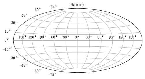
Hammer映射程序如下：

plt.figure()
plt.subplot(projection="hammer")
plt.title("Hammer")
plt.grid(True)

Hammer画图结果如下：

Lambert映射程序如下：

plt.figure()
plt.subplot(projection="lambert")
plt.title("Lambert")
plt.grid(True)

Lambert画图结果如下：

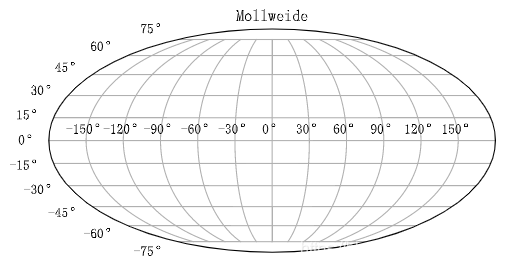
Mollweide映射程序如下：

plt.figure()
plt.subplot(projection="mollweide")
plt.title("Mollweide")
plt.grid(True)

Mollweide画图结果如下：

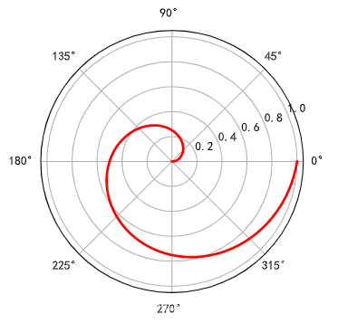
最后介绍一种最常用的映射即polar映射，也就是极坐标系，polar映射映射程序如下：

radi = np.linspace(0, 1, 100)
theta = 2*np.pi*radi

ax = plt.subplot(111, polar=True)
ax.plot(theta, radi, color='r', lw=2)
plt.show()

polar画图结果如下：

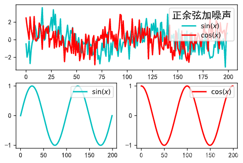
3.3.2综合示例

ax = plt.subplot(2, 2, (1, 2))
ax.plot(y+np.random.randn(200), ls='-', lw=2, color='c', label=r'$\sin(x)$')
ax.plot(y1+np.random.randn(200), ls='-', lw=2, color='r', label=r'$\cos(x)$')
ax.legend(title='正余弦加噪声', title_fontsize=15, loc='upper right')

ax = plt.subplot(2, 2, 3)
ax.plot(y, ls='-', lw=2, color='c', label=r'$\sin(x)$')
ax.legend(loc='upper right')

ax = plt.subplot(2, 2, 4)
ax.plot(y1, ls='-', lw=2, color='r', label=r'$\cos(x)$')
ax.legend(loc='upper right')

plt.show()

其画图结果如下：

---

四.add_subplots函数

这个方法是Figure类的类方法也是上面两个函数的最重要的内部实现函数。

4.1函数定义

add_subplot(nrows, ncols, index, **kwargs)
           add_subplot(pos, **kwargs)
           add_subplot(ax)
           add_subplot()

add_subplots函数的参数同plt.subplot方法的参数几乎一致，再次就不在赘述了，可以看上文的plt.subplot函数的介绍。

4.2函数讲解

该方法最大的特点就是作为类方法，其使用必须要有相应的实例，而不是像其他两个函数一样都是用gcf()方法调用当前Figure对象，这就是说我们可以在多个Figure对象上进行操作，精确创建不同对象上的分图。

4.3函数示例

4.3.1综合示例

程序展示了如何精确的创建两个Figure对象上的分图，示例程序如下：

import matplotlib.pyplot as plt
import numpy as np
import matplotlib as mpl


mpl.rcParams['font.sans-serif'] = ['SimHei']
mpl.rcParams['axes.unicode_minus'] = False

fig1 = plt.figure(num=1)
fig2 = plt.figure(num=2)
x = np.linspace(-2*np.pi, 2*np.pi, 200)
y = np.sin(x)
y1 = np.cos(x)

ax = fig1.add_subplot(2, 2, (1, 2))
ax.plot(y+np.random.randn(200), ls='-', lw=2, color='c', label=r'$\sin(x)$')
ax.plot(y1+np.random.randn(200), ls='-', lw=2, color='r', label=r'$\cos(x)$')
ax.legend(title='正余弦加噪声', title_fontsize=15, loc='upper right')

ax = fig1.add_subplot(2, 2, 3)
ax.plot(y, ls='-', lw=2, color='c', label=r'$\sin(x)$')
ax.legend(loc='upper right')

ax = fig1.add_subplot(2, 2, 4)
ax.plot(y1, ls='-', lw=2, color='r', label=r'$\cos(x)$')
ax.legend(loc='upper right')


x = np.linspace(0, 2 * np.pi, 500)
y = np.sin(x)*np.exp(-x)

ax = fig2.add_subplot(1, 2, 1, title='子图1')
ax.plot(x, y, 'k--', lw=2)
ax.set_title('折线图')

ax = fig2.add_subplot(1, 2, 2, title='子图2')
ax.scatter(x, y, s=10, c='skyblue', marker='o')
ax.set_title('散点图')

fig2.subplots_adjust(top=0.8)

plt.show()

其画图结果如下：

---

五.总结

个人认为最常用肯定是add_subplot方法和plt.subplots方法，一般情况下创建子区不会使用plt.subplot方法，他的用处在于检索而不是创建。假设需要精确控制创建子区的Figure对象，则使用add_subplot方法进行创建，通常学习或者简单绘图的话则考虑直接使用plt.subplots方法。

---

六.参考

1. 可视化解决方案
2. 可视化之路

---