当前位置:网站首页>YOLOv5的Tricks | 【Trick11】在线模型训练可视化工具wandb(Weights & Biases)
YOLOv5的Tricks | 【Trick11】在线模型训练可视化工具wandb(Weights & Biases)
2022-08-10 23:48:00 【Clichong】
如有错误,恳请指出。
与其说是yolov5的训练技巧,这篇博客更多的记录如何使用wandb这个在线模型训练可视化工具,感受到了yolov5作者对其的充分喜爱。
所以下面内容更多的记录下如何最简单的使用这个工具,而不是在介绍他在yolov5中的使用,后者具体可以见官方资料:Weights & Biases with YOLOv5
1. W&B简单介绍
Wandb是Weights & Biases的缩写,这款工具能够帮助跟踪你的机器学习项目。它能够自动记录模型训练过程中的超参数和输出指标,然后可视化和比较结果,并快速与同事共享结果。(感受到了yolov5作者对其极大的喜爱)
wandb和tensorboard最大区别是tensorboard的数据是存在本地的,wandb是存在wandb远端服务器,wandb会为开发真创建一个账户并生成登陆api的key。运行自己程序之前需要先登陆wandb。
在之前我也稍微介绍过Visdom与tensorboard的使用,见下面两个链接:
还介绍过普通的日志记录工具:
如果是简单的想记录中间训练过程的结果,其实wandb和以上提到的两种可视化工具是差不多的,甚至还可以讲训练结果与中间过程结果保存的本地直接查看(logging日志处理),但是wandb好像可以提供更多强悍的功能。其功能如下:
- Dashboard:Track experiments(跟踪实验), visualize results(可视化结果);
- Reports:Save and share reproducible findings(分享和保存结果);
- Sweeps:Optimize models with hyperparameter tuning(超参调优);
- Artifacts:Dataset and model versioning, pipeline tracking(数据集和模型的版本控制);
通过wandb,能够给你的机器学习项目带来强大的交互式可视化调试体验,能够自动化记录Python脚本中的图标,并且实时在网页仪表盘展示它的结果,例如,损失函数、准确率、召回率,它能够让你在最短的时间内完成机器学习项目可视化图片的制作。(这一点还是值得使用的,比自己记录数据然后matplotlib进行绘图要方便的多,还是推荐使用这些可视化的工具来减少不必要的代码编写,之前我就是憨批的自己matplotlib绘图的…)
- 核心优点
wandb并不单纯的是一款数据可视化工具。它具有更为强大的模型和数据版本管理。此外,还可以对你训练的模型进行调优。
wandb另外一大亮点的就是强大的兼容性,它能够和Jupyter、TensorFlow、Pytorch、Keras、Scikit、fast.ai、LightGBM、XGBoost一起结合使用。
因此,它不仅可以给你带来时间和精力上的节省,还能够给你的结果带来质的改变。
但是,wandb的高级功能对我来说暂时还用不上,等之后接触到的时候再查看,下面记录的是他的一些简单的可视化结果与保存结果的功能实现。
2. W&B快速入门
以下测试环境,全部是在本地远程调用服务器的jupyter notebook上进行。
- 安装库
pip install wandb
- 创建用户
wandb login
注册界面:https://wandb.ai/,然后把对应的key复制下来填写,就可以了
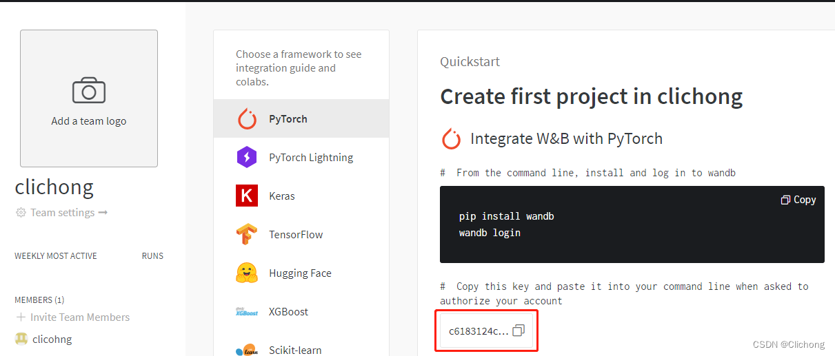
过程如下:
(yolo) [@localhost ~]$ wandb login
wandb: Logging into wandb.ai. (Learn how to deploy a W&B server locally: https://wandb.me/wandb-server)
wandb: You can find your API key in your browser here: https://wandb.ai/authorize
wandb: Paste an API key from your profile and hit enter, or press ctrl+c to quit:
wandb: Appending key for api.wandb.ai to your netrc file: /home/xxx/.netrc
- 初始化
# Inside my model training code
import wandb
wandb.init(project="my-project")
此时,就会弹出云端的对应链接,所以其和jupyter是兼容的,可以直接内置查看这个网页
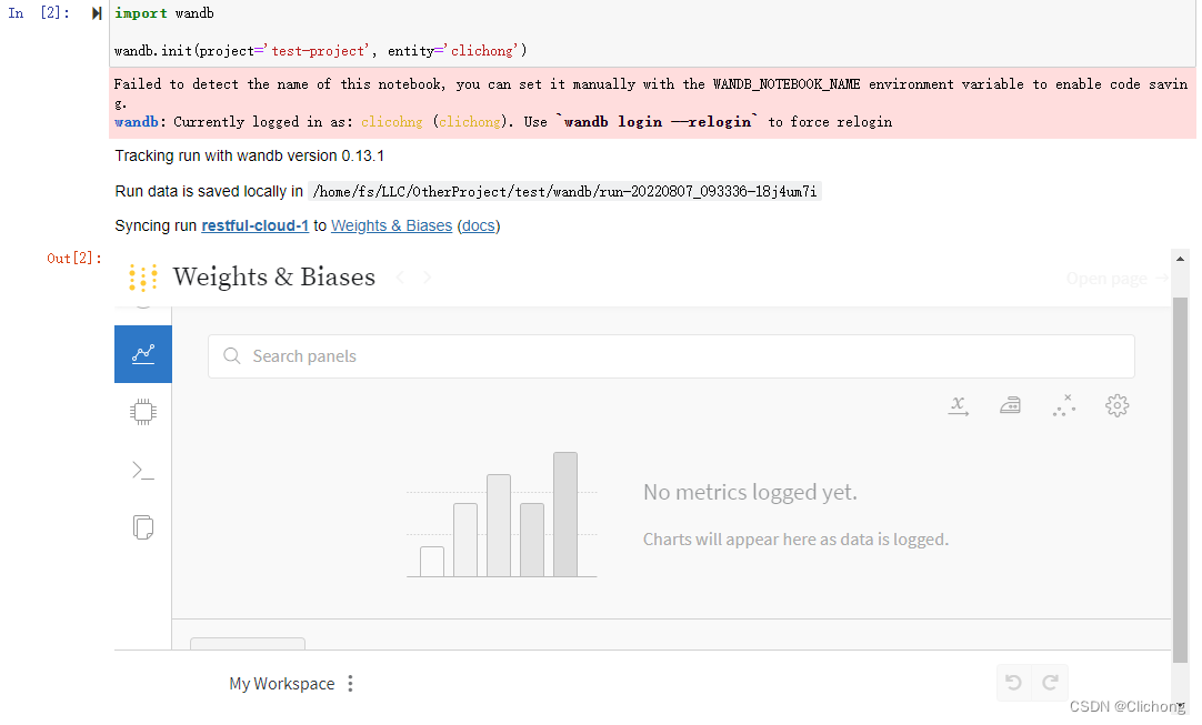
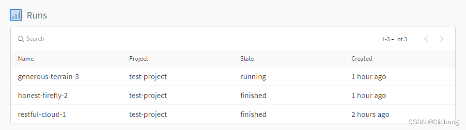
在wandb的home界面就会显示此时正在进行的进程
- 声明超参数
# config is a variable that holds and saves hyper parameters and inputs
config = wandb.config  # Initialize config
config.batch_size = 4  # input batch size for training (default:64)
config.test_batch_size = 10  # input batch size for testing(default:1000)
config.epochs = 10  # number of epochs to train(default:10)
config.lr = 0.1  # learning rate(default:0.01)
config.momentum = 0.1  # SGD momentum(default:0.5)
config.no_cuda = False  # disables CUDA training
config.seed = 42  # random seed(default:42)
config.log_interval = 10  # how many batches to wait before logging training status
- 记录日志
# wandb.log用来记录一些日志(accuracy,loss and epoch), 便于随时查看网路的性能
def test(args, model, device, test_loader, classes):
    model.eval()
    # switch model to evaluation mode.
    # This is necessary for layers like dropout, batchNorm etc. which behave differently in training and evaluation mode
    test_loss = 0
    correct = 0
    example_images = []

    with torch.no_grad():
        for data, target in test_loader:
            # Load the input features and labels from the test dataset
            data, target = data.to(device), target.to(device)

            # Make predictions: Pass image data from test dataset,
            # make predictions about class image belongs to(0-9 in this case)
            output = model(data)

            # Compute the loss sum up batch loss
            test_loss += F.nll_loss(output, target, reduction='sum').item()

            # Get the index of the max log-probability
            pred = output.max(1, keepdim=True)[1]
            correct += pred.eq(target.view_as(pred)).sum().item()

            # Log images in your test dataset automatically,
            # along with predicted and true labels by passing pytorch tensors with image data into wandb.
            example_images.append(wandb.Image(
                data[0], caption="Pred:{} Truth:{}".format(classes[pred[0].item()], classes[target[0]])))

   # wandb.log(a_dict) logs the keys and values of the dictionary passed in and associates the values with a step.
   # You can log anything by passing it to wandb.log(),
   # including histograms, custom matplotlib objects, images, video, text, tables, html, pointclounds and other 3D objects.
   # Here we use it to log test accuracy, loss and some test images (along with their true and predicted labels).
    wandb.log({

        "Examples": example_images,
        "Test Accuracy": 100. * correct / len(test_loader.dataset),
        "Test Loss": test_loss
    })
其实,主要就是中间结果运行完之后。添加在wandb.log上,也就是最后的几行代码:
# 数据传入
wandb.log({

        "Examples": example_images,
        "Test Accuracy": 100. * correct / len(test_loader.dataset),
        "Test Loss": test_loss
    })

# 图像传入
wandb.log({
    "examples" : [wandb.Image(i) for i in images]})
- 保存文件
# by default, this will save to a new subfolder for files associated
# with your run, created in wandb.run.dir (which is ./wandb by default)
wandb.save("mymodel.h5")

# you can pass the full path to the Keras model API
model.save(os.path.join(wandb.run.dir, "mymodel.h5"))
使用wandb以后,模型输出,log和要保存的文件将会同步到cloud。
3. W&B使用示例
以一个最简单的神经网络,进行一个cifar10的十分类任务为例来展示wandb的用法,代码来自参考资料3,亲测可用。代码比较简单,就不作解释了,使用的时候设置一下cifar10对应的数据集存放路径即可。
- 参考代码
from __future__ import print_function
import argparse
import random  # to set the python random seed
import numpy  # to set the numpy random seed
import torch
import torch.nn as nn
import torch.nn.functional as F
import torch.optim as optim
from torchvision import datasets, transforms
from torch.utils.data import DataLoader
# Ignore excessive warnings
import logging
logging.propagate = False
logging.getLogger().setLevel(logging.ERROR)

# WandB – Import the wandb library
import wandb
# WandB – Login to your wandb account so you can log all your metrics

# 定义Convolutional Neural Network:

class Net(nn.Module):
    def __init__(self):
        super(Net, self).__init__()

        # In our constructor, we define our neural network architecture that we'll use in the forward pass.
        # Conv2d() adds a convolution layer that generates 2 dimensional feature maps
        # to learn different aspects of our image.
        self.conv1 = nn.Conv2d(3, 6, kernel_size=5)
        self.conv2 = nn.Conv2d(6, 16, kernel_size=5)

        # Linear(x,y) creates dense, fully connected layers with x inputs and y outputs.
        # Linear layers simply output the dot product of our inputs and weights.
        self.fc1 = nn.Linear(16 * 5 * 5, 120)
        self.fc2 = nn.Linear(120, 84)
        self.fc3 = nn.Linear(84, 10)

    def forward(self, x):
        # Here we feed the feature maps from the convolutional layers into a max_pool2d layer.
        # The max_pool2d layer reduces the size of the image representation our convolutional layers learnt,
        # and in doing so it reduces the number of parameters and computations the network needs to perform.
        # Finally we apply the relu activation function which gives us max(0, max_pool2d_output)
        x = F.relu(F.max_pool2d(self.conv1(x), 2))
        x = F.relu(F.max_pool2d(self.conv2(x), 2))

        # Reshapes x into size (-1, 16 * 5 * 5)
        # so we can feed the convolution layer outputs into our fully connected layer.
        x = x.view(-1, 16 * 5 * 5)

        # We apply the relu activation function and dropout to the output of our fully connected layers.
        x = F.relu(self.fc1(x))
        x = F.relu(self.fc2(x))
        x = self.fc3(x)

        # Finally we apply the softmax function to squash the probabilities of each class (0-9)
        # and ensure they add to 1.
        return F.log_softmax(x, dim=1)

def train(config, model, device, train_loader, optimizer, epoch):
    # switch model to training mode. This is necessary for layers like dropout, batchNorm etc.
    # which behave differently in training and evaluation mode.
    model.train()

    # we loop over the data iterator, and feed the inputs to the network and adjust the weights.
    for batch_id, (data, target) in enumerate(train_loader):
        if batch_id > 20:
            break
        # Loop the input features and labels from the training dataset.
        data, target = data.to(device), target.to(device)

        # Reset the gradients to 0 for all learnable weight parameters
        optimizer.zero_grad()

        # Forward pass: Pass image data from training dataset, make predictions
        # about class image belongs to (0-9 in this case).
        output = model(data)

        # Define our loss function, and compute the loss
        loss = F.nll_loss(output, target)

        # Backward pass:compute the gradients of loss,the model's parameters
        loss.backward()

        # update the neural network weights
        optimizer.step()


# wandb.log用来记录一些日志(accuracy,loss and epoch), 便于随时查看网路的性能
def test(args, model, device, test_loader, classes):
    model.eval()
    # switch model to evaluation mode.
    # This is necessary for layers like dropout, batchNorm etc. which behave differently in training and evaluation mode
    test_loss = 0
    correct = 0
    example_images = []

    with torch.no_grad():
        for data, target in test_loader:
            # Load the input features and labels from the test dataset
            data, target = data.to(device), target.to(device)

            # Make predictions: Pass image data from test dataset,
            # make predictions about class image belongs to(0-9 in this case)
            output = model(data)

            # Compute the loss sum up batch loss
            test_loss += F.nll_loss(output, target, reduction='sum').item()

            # Get the index of the max log-probability
            pred = output.max(1, keepdim=True)[1]
            correct += pred.eq(target.view_as(pred)).sum().item()

            # Log images in your test dataset automatically,
            # along with predicted and true labels by passing pytorch tensors with image data into wandb.
            example_images.append(wandb.Image(
                data[0], caption="Pred:{} Truth:{}".format(classes[pred[0].item()], classes[target[0]])))

   # wandb.log(a_dict) logs the keys and values of the dictionary passed in and associates the values with a step.
   # You can log anything by passing it to wandb.log(),
   # including histograms, custom matplotlib objects, images, video, text, tables, html, pointclounds and other 3D objects.
   # Here we use it to log test accuracy, loss and some test images (along with their true and predicted labels).
    wandb.log({

        "Examples": example_images,
        "Test Accuracy": 100. * correct / len(test_loader.dataset),
        "Test Loss": test_loss
    })

# 初始化一个wandb run, 并设置超参数
# Initialize a new run
# wandb.init(project="pytorch-intro")
wandb.init(project='test-project', entity='clichong')
wandb.watch_called = False  # Re-run the model without restarting the runtime, unnecessary after our next release

# config is a variable that holds and saves hyper parameters and inputs
config = wandb.config  # Initialize config
config.batch_size = 4  # input batch size for training (default:64)
config.test_batch_size = 10  # input batch size for testing(default:1000)
config.epochs = 10  # number of epochs to train(default:10)
config.lr = 0.1  # learning rate(default:0.01)
config.momentum = 0.1  # SGD momentum(default:0.5)
config.no_cuda = False  # disables CUDA training
config.seed = 42  # random seed(default:42)
config.log_interval = 10  # how many batches to wait before logging training status


def main():
    use_cuda = not config.no_cuda and torch.cuda.is_available()
    device = torch.device("cuda:0" if use_cuda else "cpu")
    kwargs = {
    'num_workers': 1, 'pin_memory': True} if use_cuda else {
    }

    # Set random seeds and deterministic pytorch for reproducibility
    # random.seed(config.seed) # python random seed
    torch.manual_seed(config.seed)  # pytorch random seed
    # numpy.random.seed(config.seed) # numpy random seed
    torch.backends.cudnn.deterministic = True

    # Load the dataset: We're training our CNN on CIFAR10.
    # First we define the transformations to apply to our images.
    transform = transforms.Compose([
        transforms.ToTensor(),
        transforms.Normalize((0.5, 0.5, 0.5), (0.5, 0.5, 0.5))
    ])

    # Now we load our training and test datasets and apply the transformations defined above
    train_loader = DataLoader(datasets.CIFAR10(
        root='../../Classification/StageCNN/dataset/cifar10/',  # 路径自行更改
        train=True,
        download=False,
        transform=transform
    ), batch_size=config.batch_size, shuffle=True, **kwargs)

    test_loader = DataLoader(datasets.CIFAR10(
        root='../../Classification/StageCNN/dataset/cifar10/',  # 路径自行更改
        train=False,
        download=False,
        transform=transform
    ), batch_size=config.batch_size, shuffle=False, **kwargs)

    classes = ('plane', 'car', 'bird', 'cat', 'deer', 'dog', 'frog', 'horse', 'ship', 'truck')
    # Initialize our model, recursively go over all modules and convert their parameters
    # and buffers to CUDA tensors (if device is set to cuda)
    model = Net().to(device)
    optimizer = optim.SGD(model.parameters(), lr=config.lr, momentum=config.momentum)

    # wandb.watch() automatically fetches all layer dimensions, gradients, model parameters
    # and logs them automatically to your dashboard.
    # using log="all" log histograms of parameter values in addition to gradients
    wandb.watch(model, log="all")
    for epoch in range(1, config.epochs + 1):
        train(config, model, device, train_loader, optimizer, epoch)
        test(config, model, device, test_loader, classes)

    # Save the model checkpoint. This automatically saves a file to the cloud
    torch.save(model.state_dict(), 'model.h5')
    wandb.save('model.h5')


if __name__ == '__main__':
    main()
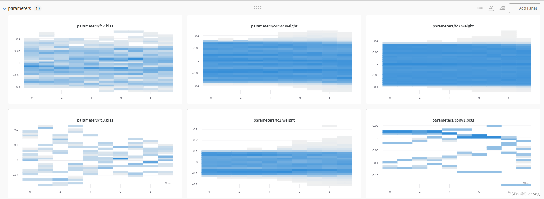
- Parameters
在运行当中,可以在其提供的链接中动态的查看训练过程与中间结果,wandb.watch(model, log="all") 可以自动获取所有层尺寸、梯度、模型参数,并将它们自动记录到云端的仪表板中。如下所示:
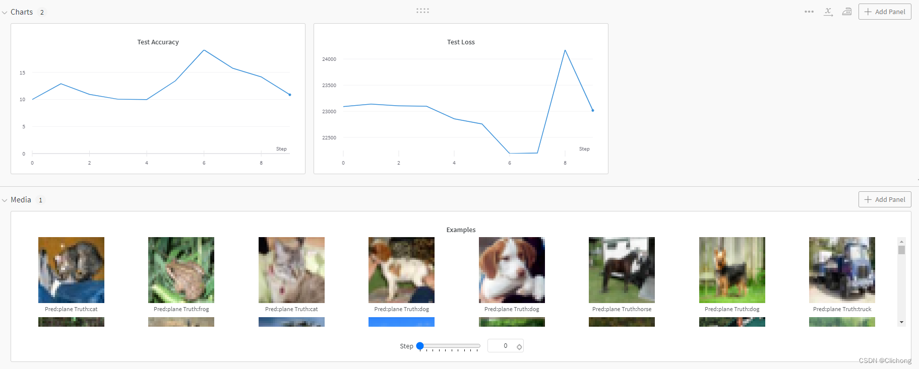
- Chart & Media
在记录中间的测试准确率和测试损失时,还可以把测试的图像列表保存下来存放在云端,很方便。
# example_images.append(wandb.Image(
# data[0], caption="Pred:{} Truth:{}".format(classes[pred[0].item()], classes[target[0]])))

wandb.log({

        "Examples": example_images,
        "Test Accuracy": 100. * correct / len(test_loader.dataset),
        "Test Loss": test_loss
    })
云端结果显示如下:
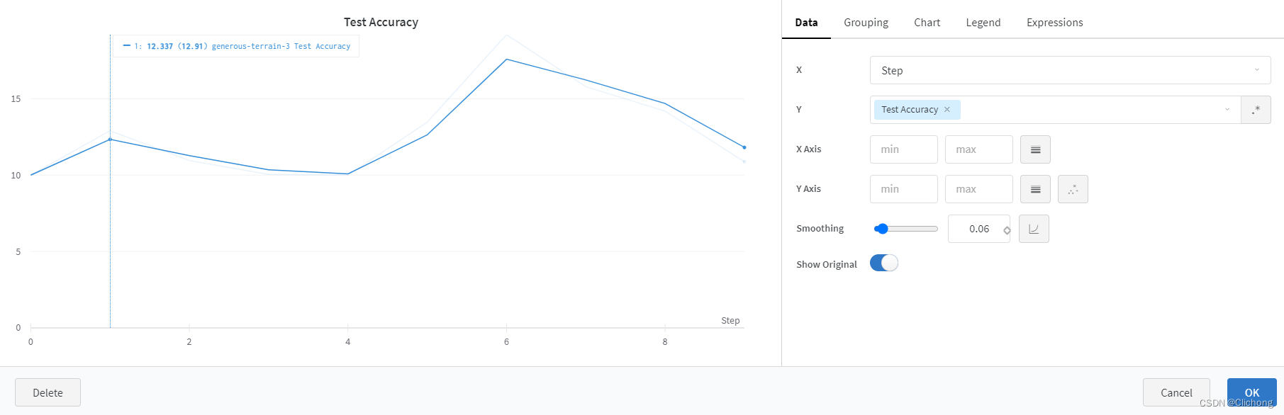
还可以单独图表进行分析与平滑等处理:
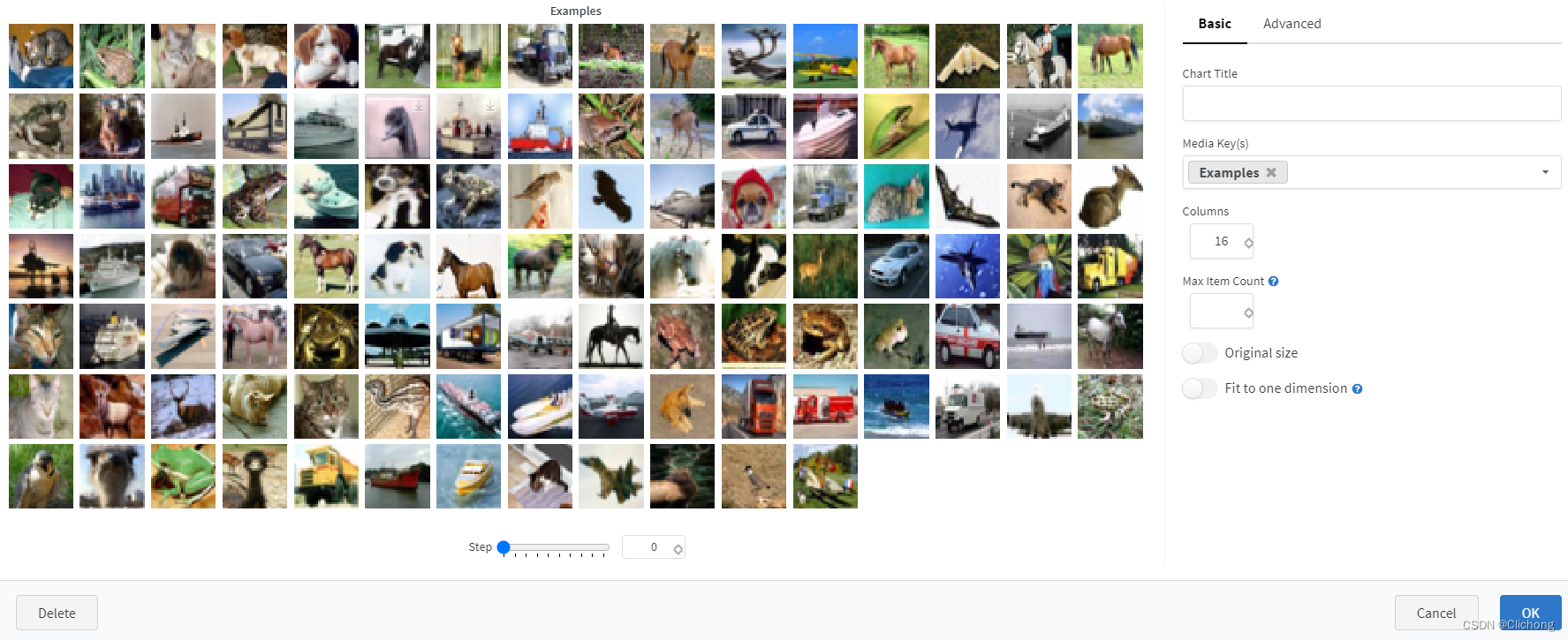
上传的图像也可以进行设置:
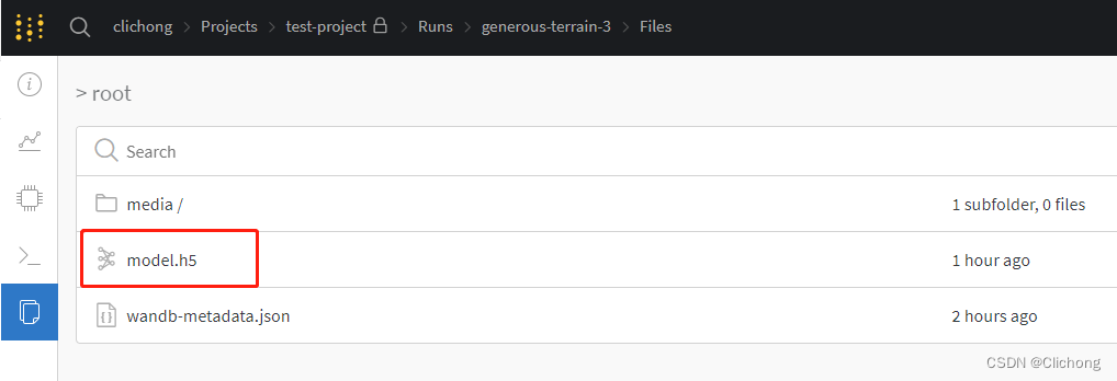
- Save
在模型训练完成保存在本地上时,还可以进行 wandb.save('model.h5') ,将模型保存在云端上,可以在相关路径下找到保存的模型。
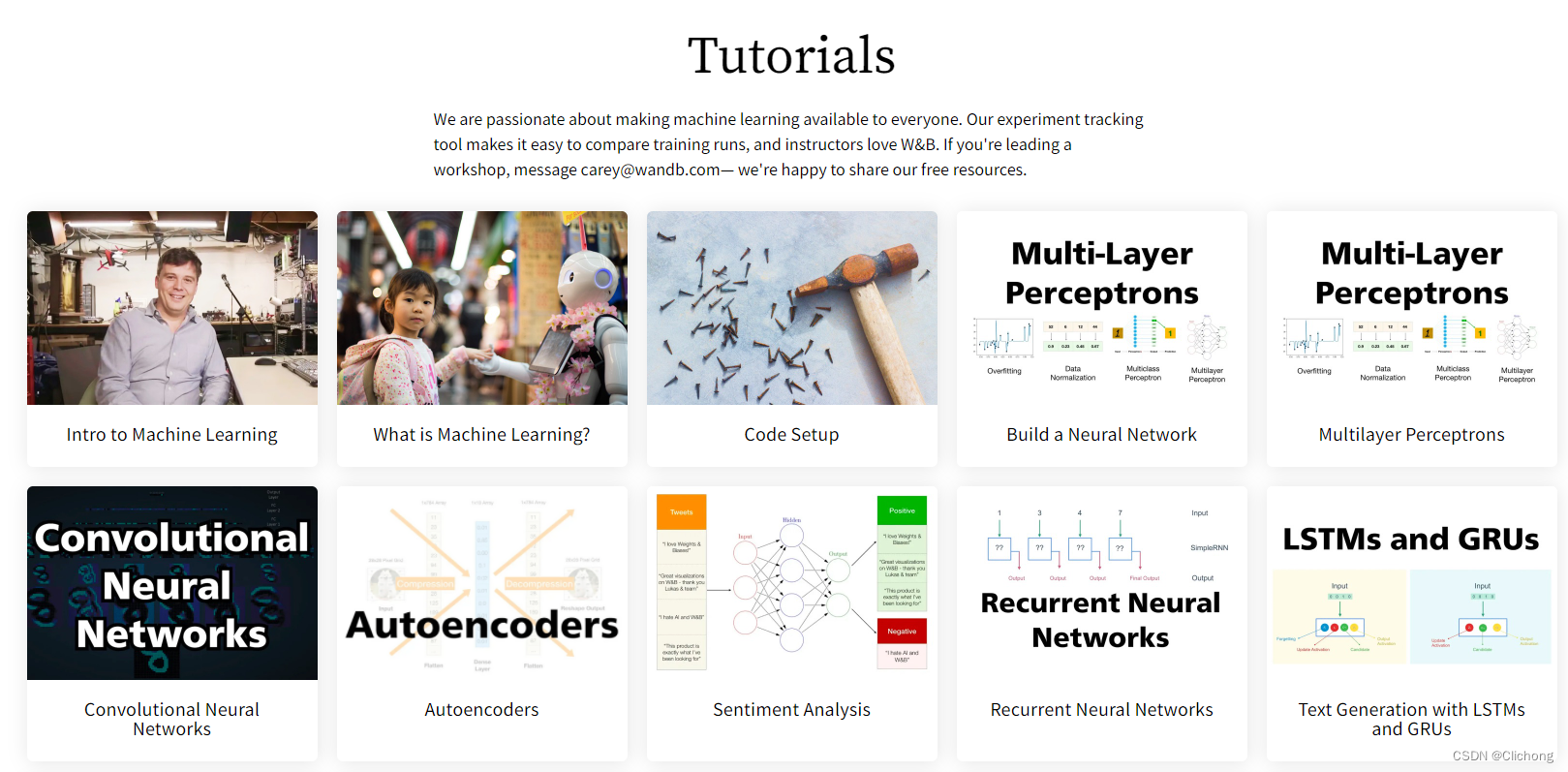
4. W&B更多帮助
在W&B的官网中,还有更多的示例和更多的教程,更良心的是支持中文,简直爱了。
官方文档资料:https://docs.wandb.ai/v/zh-hans/examples
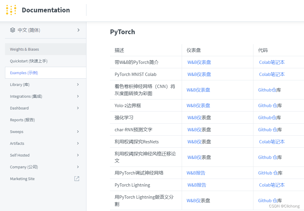
官方教程资料:https://wandb.ai/site/tutorials
参考资料:
边栏推荐
猜你喜欢
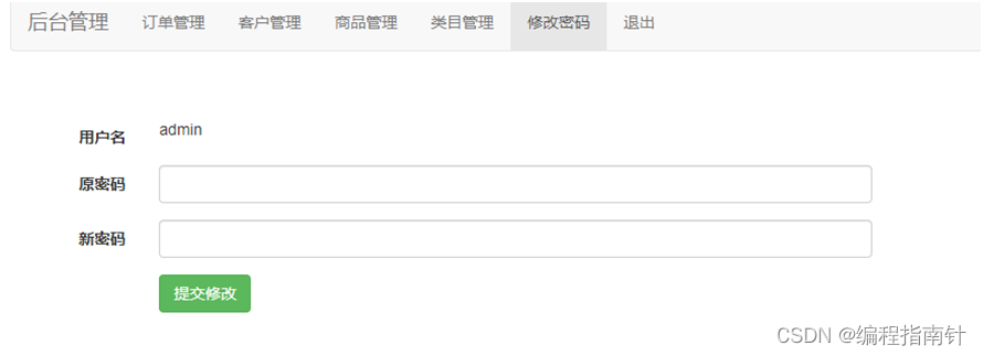
Web-based meal ordering system in epidemic quarantine area
10. Notes on receiving parameters
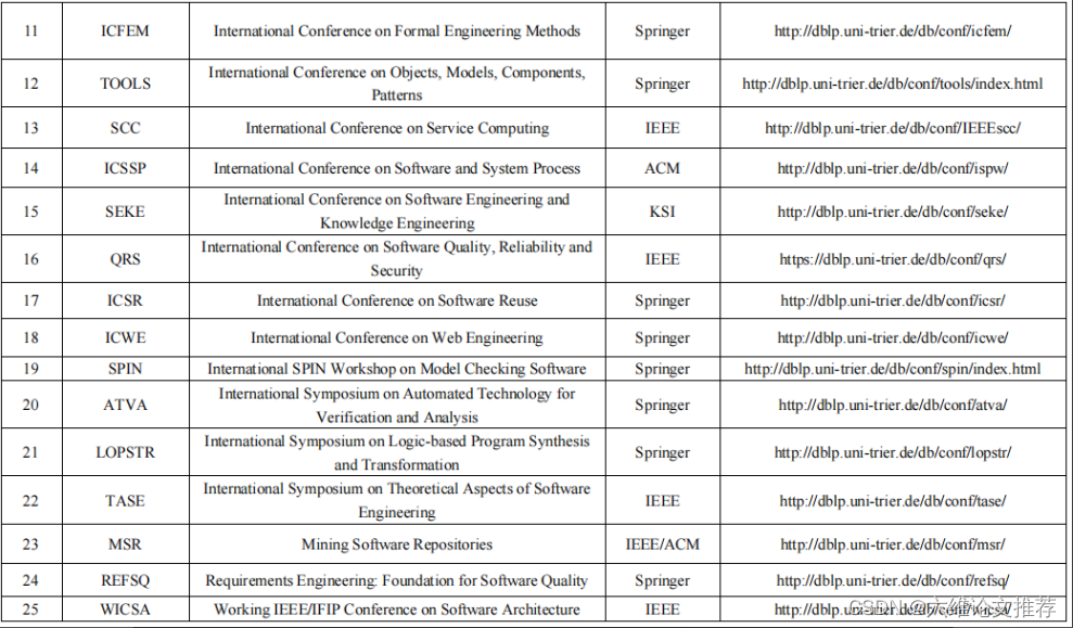
Which foreign language journals and conferences can be submitted for software engineering/system software/programming language?
Based on the SSM to reach the phone sales mall system
Deep Learning Transformer Architecture Analysis
![[C language] First understanding of pointers](/img/f2/3e28381212beabae85b832526808d2.png)
[C language] First understanding of pointers
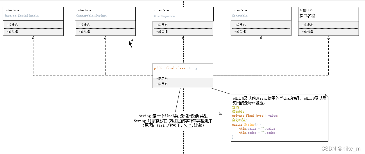
String
“蔚来杯“2022牛客暑期多校训练营2 DGHJKL题解
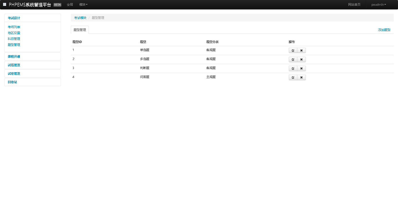
Pagoda Test-Building PHP Online Mock Exam System

iNFTnews | Web3时代,用户将拥有数据自主权
随机推荐
14. Thymeleaf
编程语言为什么有变量类型这个概念?
How to recover deleted files from the recycle bin, two methods of recovering files from the recycle bin
[Excel知识技能] 将“假“日期转为“真“日期格式
The Missing Semester of Your CS Education
CDN原理与应用简要介绍
翻译软件哪个准确度高【免费】
Special class and type conversion
11. Custom Converter
13. Content Negotiation
12. 处理 JSON
Design and implementation of flower online sales management system
电脑桌面删除的文件回收站没有,电脑上桌面删除文件在回收站找不到怎么办
软件测试证书(1)—— 软件评测师
[C] the C language program design, dynamic address book (order)
逮到一个阿里 10 年老 测试开发,聊过之后收益良多...
2. 依赖管理和自动配置
HGAME 2022 Final Pokemon v2 writeup
基于SSM实现手机销售商城系统
SAS数据处理技术(一)