当前位置:网站首页>[image classification] reproduce senet with the shortest code. Xiaobai must be collected (keras, tensorflow2. X)
[image classification] reproduce senet with the shortest code. Xiaobai must be collected (keras, tensorflow2. X)
2022-04-23 00:23:00 【AI Xiaohao】
Catalog
Abstract
Two 、SENet Detailed explanation of structure composition
3、 ... and 、 Detailed calculation process
SENet Application in specific network ( Code implementation SE_ResNet)
The first residual module
The second residual module
ResNet18、ResNet34 Complete code for the model
ResNet50、ResNet101、ResNet152 Complete code
Abstract
One 、SENet summary
Squeeze-and-Excitation Networks( abbreviation SENet) yes Momenta Hu Jie team (WMW) A new network structure is proposed , utilize SENet, Win the last ImageNet 2017 competition Image Classification The champion of the mission , stay ImageNet There will be top-5 error Down to 2.251%, The original best result was 2.991%.
The author will SENet block Plug into the existing classification network , We have achieved good results . The author's motivation is to explicitly model the interdependencies between feature channels . in addition , The author does not introduce a new spatial dimension to fuse feature channels , But with a brand new 「 Feature recalibration 」 Strategy . say concretely , It is to automatically obtain the importance of each feature channel through learning , Then according to this importance, we can promote the useful features and suppress the features that are not useful for the current task .
In layman's terms SENet The core idea of the Internet is based on loss To learn feature weights , To make effective feature map Great power , Ineffective or ineffective feature map The training model with small weight can achieve better results .SE block Embedded in some original classification networks, some parameters and computation are inevitably added , But in the face of the effect is still acceptable .Sequeeze-and-Excitation(SE) block It's not a complete network structure , It's a substructure , It can be embedded in other classification or detection models .
Two 、SENet Detailed explanation of structure composition
In the above structure ,Squeeze and Excitation It's two very critical operations , The following is a detailed description of .

Above, SE Schematic diagram of the module . Given an input x, The number of characteristic channels is  , Through a series of convolutions and other general transformations, we get a characteristic channel number of C Characteristics of . The previously obtained features are also re marked through the following three operations :
1、Squeeze operation , Feature compression along spatial dimensions , Turn each two-dimensional feature channel into a real number , This real number has a global receptive field to some extent , And the dimension of output matches the number of characteristic channels of input . It represents the global distribution of the response on the characteristic channel , Moreover, the layer close to the input can also obtain the global receptive field , This is very useful in many tasks .
2、 Excitation operation , It's a mechanism similar to that of a gate in a recurrent neural network . Through parameters w To generate weights for each feature channel , The parameter w It is learned to explicitly model the correlation between feature channels .
3、 Reweight operation , take Excitation The weight of the output is regarded as the importance of each feature channel after feature selection , Then, by multiplication, it is weighted to the previous features one by one , Complete the recalibration of the original feature on the channel dimension .
3、 ... and 、 Detailed calculation process
First  This step is the conversion operation ( Strictly speaking, it does not belong to SENet, It belongs to the original network , You can look at the back SENet and Inception And ResNet The combination of the Internet ), In this paper, it is just a standard convolution operation , The definition of input and output is as follows :

So this The formula is the following formula 1( Convolution operation , It means the first one c Convolution kernels ,
 It means the first one s Inputs ).

Got U Namely Figure1 The second three-dimensional matrix on the left in , Also called tensor, Or call it C Size is H*W Of feature map. and uc Express U pass the civil examinations c Two dimensional matrix , Subscript c Express channel.
The next step is Squeeze operation , The formula is very simple , It's just one. global average pooling:

So the formula 2 will H*W*C The input is converted to 1*1*C Output , Corresponding Figure1 Medium Fsq operation . Why is there such a step ? The result of this step is equivalent to showing that the layer C individual feature map The numerical distribution of , Or global information .
The next step is Excitation operation , As formula 3. Look directly at the last equal sign , front squeeze And what you get is z, Use it here first W1 multiply z, It's a full connection layer operation ,W1 The dimension of is C/r * C, This r It's a scaling parameter , In the text, I take 16, The purpose of this parameter is to reduce channel So the amount of computation is reduced . Again because z The dimension of is 1*1*C, therefore W1z The result is that 1*1*C/r; And then there's another ReLU layer , The dimension of the output remains unchanged ; And then with W2 Multiply , and W2 Multiplication is also a fully connected process ,W2 The dimension of is C*C/r, So the dimension of output is 1*1*C; And finally through sigmoid function , obtain s:
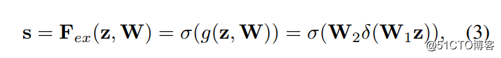
In other words, the last one s The dimension of is 1*1*C,C Express channel number . This s In fact, it is the core of this article , It's used to depict tensor U in C individual feature map The weight of . And this weight is obtained by learning from the previous fully connected layer and nonlinear layer , So you can end-to-end Training . This is the role of the integration of the two channels feature map Information , Because of the squeeze It's all in a certain place channel Of feature map Inside operation .
Get in s after , You can change the original tensor U Operation , Here's the formula 4. It's also very simple. , Namely channel-wise multiplication, What does that mean ? It's a two-dimensional matrix ,
 Is a number , Weight , So it's equivalent to Every value in the matrix is multiplied by . Corresponding Figure1 Medium Fscale.
SENet Application in specific network ( Code implementation SE_ResNet)
After introducing the concrete formula realization , Here's how SE block How to apply it to the specific network .


The picture above is about SE Module embedded in Inception An example of structure . The dimension information next to the box represents the output of the layer .
Here we use global average pooling As Squeeze operation . And then two Fully Connected Layers make up a Bottleneck Structure to model the correlation between channels , And output the same number of weights as the input features . We first reduce the feature dimension to the input 1/16, And then pass by ReLu Activate and then pass through a Fully Connected Layers rise back to the original dimension . It's better to do this than to use a Fully Connected The advantage of layers is :
1) It has more nonlinearity , It can better fit the complex correlation between channels ;
2) It greatly reduces the amount of parameters and calculation . And then through a Sigmoid The door to gain 0~1 Normalized weight between , Finally, a Scale Operation to weight the normalized weight to the characteristics of each channel .
besides ,SE Modules can also be embedded into the containing skip-connections In the module . The picture on the right is a picture of will SE Embedded in ResNet An example in the module , The operation process is basically SE-Inception equally , It's just that Addition Front to branch Residual The features of are recalibrated . If the Addition The features on the rear main branch are recalibrated , Because of the presence of 0~1 Of scale operation , Deep in the network BP When optimizing, gradient dissipation will easily occur near the input layer , It makes the model difficult to optimize .
At present, most of the mainstream networks are based on these two similar units repeat To construct by means of superposition . thus it can be seen ,SE Modules can be embedded in almost all current network structures . Through... In the original network structure building block Embed... In the unit SE modular , We can get different kinds of SENet. Such as SE-BN-Inception、SE-ResNet、SE-ReNeXt、SE-Inception-ResNet-v2 wait .
This example implements SE-ResNet, To show how SE Module embedded in ResNet In the network .SE-ResNet The model is shown in the following figure. :

The first residual module
The first residual module is used to implement ResNet18、ResNet34 Model ,SENet Embedded behind the second convolution .
       #  The first residual module


       class

       BasicBlock(

       layers.

       Layer):


       def

       __init__(

       self,

       filter_num,

       stride

       =

       1):


       super(

       BasicBlock,

       self).

       __init__()


       self.

       conv1

       =

       layers.

       Conv2D(

       filter_num, (

       3,

       3),

       strides

       =

       stride,

       padding

       =

       'same')


       self.

       bn1

       =

       layers.

       BatchNormalization()


       self.

       relu

       =

       layers.

       Activation(

       'relu')


       self.

       conv2

       =

       layers.

       Conv2D(

       filter_num, (

       3,

       3),

       strides

       =

       1,

       padding

       =

       'same')


       self.

       bn2

       =

       layers.

       BatchNormalization()


       # se-block


       self.

       se_globalpool

       =

       keras.

       layers.

       GlobalAveragePooling2D()


       self.

       se_resize

       =

       keras.

       layers.

       Reshape((

       1,

       1,

       filter_num))


       self.

       se_fc1

       =

       keras.

       layers.

       Dense(

       units

       =

       filter_num

       /

       /

       16,

       activation

       =

       'relu',


       use_bias

       =

       False)


       self.

       se_fc2

       =

       keras.

       layers.

       Dense(

       units

       =

       filter_num,

       activation

       =

       'sigmoid',


       use_bias

       =

       False)


       if

       stride

       !=

       1:


       self.

       downsample

       =

       Sequential()


       self.

       downsample.

       add(

       layers.

       Conv2D(

       filter_num, (

       1,

       1),

       strides

       =

       stride))


       else:


       self.

       downsample

       =

       lambda

       x:

       x


       def

       call(

       self,

       input,

       training

       =

       None):


       out

       =

       self.

       conv1(

       input)


       out

       =

       self.

       bn1(

       out)


       out

       =

       self.

       relu(

       out)


       out

       =

       self.

       conv2(

       out)


       out

       =

       self.

       bn2(

       out)


       # se_block


       b

       =

       out


       out

       =

       self.

       se_globalpool(

       out)


       out

       =

       self.

       se_resize(

       out)


       out

       =

       self.

       se_fc1(

       out)


       out

       =

       self.

       se_fc2(

       out)


       out

       =

       keras.

       layers.

       Multiply()([

       b,

       out])


       identity

       =

       self.

       downsample(

       input)


       output

       =

       layers.

       add([

       out,

       identity])


       output

       =

       tf.

       nn.

       relu(

       output)


       return

       output
- 1.
- 2.
- 3.
- 4.
- 5.
- 6.
- 7.
- 8.
- 9.
- 10.
- 11.
- 12.
- 13.
- 14.
- 15.
- 16.
- 17.
- 18.
- 19.
- 20.
- 21.
- 22.
- 23.
- 24.
- 25.
- 26.
- 27.
- 28.
- 29.
- 30.
- 31.
- 32.
- 33.
- 34.
- 35.
- 36.
- 37.
- 38.
- 39.
- 40.
The second residual module
The second residual module is used to implement ResNet50、ResNet101、ResNet152 Model ,SENet The module is embedded behind the third convolution .
       #  The second residual module


       class

       Block(

       layers.

       Layer):


       def

       __init__(

       self,

       filters,

       downsample

       =

       False,

       stride

       =

       1):


       super(

       Block,

       self).

       __init__()


       self.

       downsample

       =

       downsample


       self.

       conv1

       =

       layers.

       Conv2D(

       filters, (

       1,

       1),

       strides

       =

       stride,

       padding

       =

       'same')


       self.

       bn1

       =

       layers.

       BatchNormalization()


       self.

       relu

       =

       layers.

       Activation(

       'relu')


       self.

       conv2

       =

       layers.

       Conv2D(

       filters, (

       3,

       3),

       strides

       =

       1,

       padding

       =

       'same')


       self.

       bn2

       =

       layers.

       BatchNormalization()


       self.

       conv3

       =

       layers.

       Conv2D(

       4

       *

       filters, (

       1,

       1),

       strides

       =

       1,

       padding

       =

       'same')


       self.

       bn3

       =

       layers.

       BatchNormalization()


       # se-block


       self.

       se_globalpool

       =

       keras.

       layers.

       GlobalAveragePooling2D()


       self.

       se_resize

       =

       keras.

       layers.

       Reshape((

       1,

       1,

       4

       *

       filters))


       self.

       se_fc1

       =

       keras.

       layers.

       Dense(

       units

       =

       4

       *

       filters

       /

       /

       16,

       activation

       =

       'relu',


       use_bias

       =

       False)


       self.

       se_fc2

       =

       keras.

       layers.

       Dense(

       units

       =

       4

       *

       filters,

       activation

       =

       'sigmoid',


       use_bias

       =

       False)


       if

       self.

       downsample:


       self.

       shortcut

       =

       Sequential()


       self.

       shortcut.

       add(

       layers.

       Conv2D(

       4

       *

       filters, (

       1,

       1),

       strides

       =

       stride))


       self.

       shortcut.

       add(

       layers.

       BatchNormalization(

       axis

       =

       3))


       def

       call(

       self,

       input,

       training

       =

       None):


       out

       =

       self.

       conv1(

       input)


       out

       =

       self.

       bn1(

       out)


       out

       =

       self.

       relu(

       out)


       out

       =

       self.

       conv2(

       out)


       out

       =

       self.

       bn2(

       out)


       out

       =

       self.

       relu(

       out)


       out

       =

       self.

       conv3(

       out)


       out

       =

       self.

       bn3(

       out)


       b

       =

       out


       out

       =

       self.

       se_globalpool(

       out)


       out

       =

       self.

       se_resize(

       out)


       out

       =

       self.

       se_fc1(

       out)


       out

       =

       self.

       se_fc2(

       out)


       out

       =

       keras.

       layers.

       Multiply()([

       b,

       out])


       if

       self.

       downsample:


       shortcut

       =

       self.

       shortcut(

       input)


       else:


       shortcut

       =

       input


       output

       =

       layers.

       add([

       out,

       shortcut])


       output

       =

       tf.

       nn.

       relu(

       output)


       return

       output
- 1.
- 2.
- 3.
- 4.
- 5.
- 6.
- 7.
- 8.
- 9.
- 10.
- 11.
- 12.
- 13.
- 14.
- 15.
- 16.
- 17.
- 18.
- 19.
- 20.
- 21.
- 22.
- 23.
- 24.
- 25.
- 26.
- 27.
- 28.
- 29.
- 30.
- 31.
- 32.
- 33.
- 34.
- 35.
- 36.
- 37.
- 38.
- 39.
- 40.
- 41.
- 42.
- 43.
- 44.
- 45.
- 46.
- 47.
ResNet18、ResNet34 Complete code for the model
       import

       tensorflow

       as

       tf


       from

       tensorflow

       import

       keras


       from

       tensorflow.

       keras

       import

       layers,

       Sequential


       #  The first residual module


       class

       BasicBlock(

       layers.

       Layer):


       def

       __init__(

       self,

       filter_num,

       stride

       =

       1):


       super(

       BasicBlock,

       self).

       __init__()


       self.

       conv1

       =

       layers.

       Conv2D(

       filter_num, (

       3,

       3),

       strides

       =

       stride,

       padding

       =

       'same')


       self.

       bn1

       =

       layers.

       BatchNormalization()


       self.

       relu

       =

       layers.

       Activation(

       'relu')


       self.

       conv2

       =

       layers.

       Conv2D(

       filter_num, (

       3,

       3),

       strides

       =

       1,

       padding

       =

       'same')


       self.

       bn2

       =

       layers.

       BatchNormalization()


       # se-block


       self.

       se_globalpool

       =

       keras.

       layers.

       GlobalAveragePooling2D()


       self.

       se_resize

       =

       keras.

       layers.

       Reshape((

       1,

       1,

       filter_num))


       self.

       se_fc1

       =

       keras.

       layers.

       Dense(

       units

       =

       filter_num

       /

       /

       16,

       activation

       =

       'relu',


       use_bias

       =

       False)


       self.

       se_fc2

       =

       keras.

       layers.

       Dense(

       units

       =

       filter_num,

       activation

       =

       'sigmoid',


       use_bias

       =

       False)


       if

       stride

       !=

       1:


       self.

       downsample

       =

       Sequential()


       self.

       downsample.

       add(

       layers.

       Conv2D(

       filter_num, (

       1,

       1),

       strides

       =

       stride))


       else:


       self.

       downsample

       =

       lambda

       x:

       x


       def

       call(

       self,

       input,

       training

       =

       None):


       out

       =

       self.

       conv1(

       input)


       out

       =

       self.

       bn1(

       out)


       out

       =

       self.

       relu(

       out)


       out

       =

       self.

       conv2(

       out)


       out

       =

       self.

       bn2(

       out)


       # se_block


       b

       =

       out


       out

       =

       self.

       se_globalpool(

       out)


       out

       =

       self.

       se_resize(

       out)


       out

       =

       self.

       se_fc1(

       out)


       out

       =

       self.

       se_fc2(

       out)


       out

       =

       keras.

       layers.

       Multiply()([

       b,

       out])


       identity

       =

       self.

       downsample(

       input)


       output

       =

       layers.

       add([

       out,

       identity])


       output

       =

       tf.

       nn.

       relu(

       output)


       return

       output


       class

       ResNet(

       keras.

       Model):


       def

       __init__(

       self,

       layer_dims,

       num_classes

       =

       10):


       super(

       ResNet,

       self).

       __init__()


       #  Pretreatment layer


       self.

       padding

       =

       keras.

       layers.

       ZeroPadding2D((

       3,

       3))


       self.

       stem

       =

       Sequential([


       layers.

       Conv2D(

       64, (

       7,

       7),

       strides

       =(

       2,

       2)),


       layers.

       BatchNormalization(),


       layers.

       Activation(

       'relu'),


       layers.

       MaxPool2D(

       pool_size

       =(

       3,

       3),

       strides

       =(

       2,

       2),

       padding

       =

       'same')


        ])


       # resblock


       self.

       layer1

       =

       self.

       build_resblock(

       64,

       layer_dims[

       0])


       self.

       layer2

       =

       self.

       build_resblock(

       128,

       layer_dims[

       1],

       stride

       =

       2)


       self.

       layer3

       =

       self.

       build_resblock(

       256,

       layer_dims[

       2],

       stride

       =

       2)


       self.

       layer4

       =

       self.

       build_resblock(

       512,

       layer_dims[

       3],

       stride

       =

       2)


       #  Global pooling


       self.

       avgpool

       =

       layers.

       GlobalAveragePooling2D()


       #  Fully connected layer


       self.

       fc

       =

       layers.

       Dense(

       num_classes,

       activation

       =

       tf.

       keras.

       activations.

       softmax)


       def

       call(

       self,

       input,

       training

       =

       None):


       x

       =

       self.

       padding(

       input)


       x

       =

       self.

       stem(

       x)


       x

       =

       self.

       layer1(

       x)


       x

       =

       self.

       layer2(

       x)


       x

       =

       self.

       layer3(

       x)


       x

       =

       self.

       layer4(

       x)


       # [b,c]


       x

       =

       self.

       avgpool(

       x)


       x

       =

       self.

       fc(

       x)


       return

       x


       def

       build_resblock(

       self,

       filter_num,

       blocks,

       stride

       =

       1):


       res_blocks

       =

       Sequential()


       res_blocks.

       add(

       BasicBlock(

       filter_num,

       stride))


       for

       pre

       in

       range(

       1,

       blocks):


       res_blocks.

       add(

       BasicBlock(

       filter_num,

       stride

       =

       1))


       return

       res_blocks


       def

       ResNet34(

       num_classes

       =

       10):


       return

       ResNet([

       2,

       2,

       2,

       2],

       num_classes

       =

       num_classes)


       def

       ResNet34(

       num_classes

       =

       10):


       return

       ResNet([

       3,

       4,

       6,

       3],

       num_classes

       =

       num_classes)


       model

       =

       ResNet34(

       num_classes

       =

       1000)


       model.

       build(

       input_shape

       =(

       1,

       224,

       224,

       3))


       print(

       model.

       summary())

       #  Statistical network parameters
- 1.
- 2.
- 3.
- 4.
- 5.
- 6.
- 7.
- 8.
- 9.
- 10.
- 11.
- 12.
- 13.
- 14.
- 15.
- 16.
- 17.
- 18.
- 19.
- 20.
- 21.
- 22.
- 23.
- 24.
- 25.
- 26.
- 27.
- 28.
- 29.
- 30.
- 31.
- 32.
- 33.
- 34.
- 35.
- 36.
- 37.
- 38.
- 39.
- 40.
- 41.
- 42.
- 43.
- 44.
- 45.
- 46.
- 47.
- 48.
- 49.
- 50.
- 51.
- 52.
- 53.
- 54.
- 55.
- 56.
- 57.
- 58.
- 59.
- 60.
- 61.
- 62.
- 63.
- 64.
- 65.
- 66.
- 67.
- 68.
- 69.
- 70.
- 71.
- 72.
- 73.
- 74.
- 75.
- 76.
- 77.
- 78.
- 79.
- 80.
- 81.
- 82.
- 83.
- 84.
- 85.
- 86.
- 87.
- 88.
- 89.
- 90.
- 91.
- 92.
- 93.
- 94.
- 95.
- 96.
- 97.
- 98.
- 99.
ResNet50、ResNet101、ResNet152 Complete code
       import

       tensorflow

       as

       tf


       from

       tensorflow

       import

       keras


       from

       tensorflow.

       keras

       import

       layers,

       Sequential


       #  The second residual module


       class

       Block(

       layers.

       Layer):


       def

       __init__(

       self,

       filters,

       downsample

       =

       False,

       stride

       =

       1):


       super(

       Block,

       self).

       __init__()


       self.

       downsample

       =

       downsample


       self.

       conv1

       =

       layers.

       Conv2D(

       filters, (

       1,

       1),

       strides

       =

       stride,

       padding

       =

       'same')


       self.

       bn1

       =

       layers.

       BatchNormalization()


       self.

       relu

       =

       layers.

       Activation(

       'relu')


       self.

       conv2

       =

       layers.

       Conv2D(

       filters, (

       3,

       3),

       strides

       =

       1,

       padding

       =

       'same')


       self.

       bn2

       =

       layers.

       BatchNormalization()


       self.

       conv3

       =

       layers.

       Conv2D(

       4

       *

       filters, (

       1,

       1),

       strides

       =

       1,

       padding

       =

       'same')


       self.

       bn3

       =

       layers.

       BatchNormalization()


       # se-block


       self.

       se_globalpool

       =

       keras.

       layers.

       GlobalAveragePooling2D()


       self.

       se_resize

       =

       keras.

       layers.

       Reshape((

       1,

       1,

       4

       *

       filters))


       self.

       se_fc1

       =

       keras.

       layers.

       Dense(

       units

       =

       4

       *

       filters

       /

       /

       16,

       activation

       =

       'relu',


       use_bias

       =

       False)


       self.

       se_fc2

       =

       keras.

       layers.

       Dense(

       units

       =

       4

       *

       filters,

       activation

       =

       'sigmoid',


       use_bias

       =

       False)


       if

       self.

       downsample:


       self.

       shortcut

       =

       Sequential()


       self.

       shortcut.

       add(

       layers.

       Conv2D(

       4

       *

       filters, (

       1,

       1),

       strides

       =

       stride))


       self.

       shortcut.

       add(

       layers.

       BatchNormalization(

       axis

       =

       3))


       def

       call(

       self,

       input,

       training

       =

       None):


       out

       =

       self.

       conv1(

       input)


       out

       =

       self.

       bn1(

       out)


       out

       =

       self.

       relu(

       out)


       out

       =

       self.

       conv2(

       out)


       out

       =

       self.

       bn2(

       out)


       out

       =

       self.

       relu(

       out)


       out

       =

       self.

       conv3(

       out)


       out

       =

       self.

       bn3(

       out)


       b

       =

       out


       out

       =

       self.

       se_globalpool(

       out)


       out

       =

       self.

       se_resize(

       out)


       out

       =

       self.

       se_fc1(

       out)


       out

       =

       self.

       se_fc2(

       out)


       out

       =

       keras.

       layers.

       Multiply()([

       b,

       out])


       if

       self.

       downsample:


       shortcut

       =

       self.

       shortcut(

       input)


       else:


       shortcut

       =

       input


       output

       =

       layers.

       add([

       out,

       shortcut])


       output

       =

       tf.

       nn.

       relu(

       output)


       return

       output


       class

       ResNet(

       keras.

       Model):


       def

       __init__(

       self,

       layer_dims,

       num_classes

       =

       10):


       super(

       ResNet,

       self).

       __init__()


       #  Pretreatment layer


       self.

       padding

       =

       keras.

       layers.

       ZeroPadding2D((

       3,

       3))


       self.

       stem

       =

       Sequential([


       layers.

       Conv2D(

       64, (

       7,

       7),

       strides

       =(

       2,

       2)),


       layers.

       BatchNormalization(),


       layers.

       Activation(

       'relu'),


       layers.

       MaxPool2D(

       pool_size

       =(

       3,

       3),

       strides

       =(

       2,

       2),

       padding

       =

       'same')


        ])


       # resblock


       self.

       layer1

       =

       self.

       build_resblock(

       64,

       layer_dims[

       0],

       stride

       =

       1)


       self.

       layer2

       =

       self.

       build_resblock(

       128,

       layer_dims[

       1],

       stride

       =

       2)


       self.

       layer3

       =

       self.

       build_resblock(

       256,

       layer_dims[

       2],

       stride

       =

       2)


       self.

       layer4

       =

       self.

       build_resblock(

       512,

       layer_dims[

       3],

       stride

       =

       2)


       #  Global pooling


       self.

       avgpool

       =

       layers.

       GlobalAveragePooling2D()


       #  Fully connected layer


       self.

       fc

       =

       layers.

       Dense(

       num_classes,

       activation

       =

       tf.

       keras.

       activations.

       softmax)


       def

       call(

       self,

       input,

       training

       =

       None):


       x

       =

       self.

       padding(

       input)


       x

       =

       self.

       stem(

       x)


       x

       =

       self.

       layer1(

       x)


       x

       =

       self.

       layer2(

       x)


       x

       =

       self.

       layer3(

       x)


       x

       =

       self.

       layer4(

       x)


       # [b,c]


       x

       =

       self.

       avgpool(

       x)


       x

       =

       self.

       fc(

       x)


       return

       x


       def

       build_resblock(

       self,

       filter_num,

       blocks,

       stride

       =

       1):


       res_blocks

       =

       Sequential()


       if

       stride

       !=

       1

       or

       filter_num

       *

       4

       !=

       64:


       res_blocks.

       add(

       Block(

       filter_num,

       downsample

       =

       True,

       stride

       =

       stride))


       for

       pre

       in

       range(

       1,

       blocks):


       res_blocks.

       add(

       Block(

       filter_num,

       stride

       =

       1))


       return

       res_blocks


       def

       ResNet50(

       num_classes

       =

       10):


       return

       ResNet([

       3,

       4,

       6,

       3],

       num_classes

       =

       num_classes)


       def

       ResNet101(

       num_classes

       =

       10):


       return

       ResNet([

       3,

       4,

       23,

       3],

       num_classes

       =

       num_classes)


       def

       ResNet152(

       num_classes

       =

       10):


       return

       ResNet([

       3,

       8,

       36,

       3],

       num_classes

       =

       num_classes)


       model

       =

       ResNet50(

       num_classes

       =

       1000)


       model.

       build(

       input_shape

       =(

       1,

       224,

       224,

       3))


       print(

       model.

       summary())

       #  Statistical network parameters
- 1.
- 2.
- 3.
- 4.
- 5.
- 6.
- 7.
- 8.
- 9.
- 10.
- 11.
- 12.
- 13.
- 14.
- 15.
- 16.
- 17.
- 18.
- 19.
- 20.
- 21.
- 22.
- 23.
- 24.
- 25.
- 26.
- 27.
- 28.
- 29.
- 30.
- 31.
- 32.
- 33.
- 34.
- 35.
- 36.
- 37.
- 38.
- 39.
- 40.
- 41.
- 42.
- 43.
- 44.
- 45.
- 46.
- 47.
- 48.
- 49.
- 50.
- 51.
- 52.
- 53.
- 54.
- 55.
- 56.
- 57.
- 58.
- 59.
- 60.
- 61.
- 62.
- 63.
- 64.
- 65.
- 66.
- 67.
- 68.
- 69.
- 70.
- 71.
- 72.
- 73.
- 74.
- 75.
- 76.
- 77.
- 78.
- 79.
- 80.
- 81.
- 82.
- 83.
- 84.
- 85.
- 86.
- 87.
- 88.
- 89.
- 90.
- 91.
- 92.
- 93.
- 94.
- 95.
- 96.
- 97.
- 98.
- 99.
- 100.
- 101.
- 102.
- 103.
- 104.
- 105.
- 106.
- 107.
- 108.
- 109.
版权声明
本文为[AI Xiaohao]所创,转载请带上原文链接,感谢
https://yzsam.com/2022/04/202204222322243295.html
边栏推荐
- (transfer) Aspose Introduction to DOM tree structure, node class inheritance relationship and description of words Programming Guide
- js -对连续月份数据做处理拆分
- 倍福NC轴走速度模式
- NPM and NPX view dependent package versions
- 湖泊的水色、水环境、水文遥感的区别
- 威伦触摸屏和倍福PLC通信报错AdsParseSymbol invalid array index
- 倍福scope view示波器读取组态IO的信号
- 微软官网下载Net Framework流程
- (transfer) SSH login configuration and file transfer
- npm 和 npx 查看依赖包版本
猜你喜欢
【图像分类】用最简短的代码复现SeNet,小白一定要收藏(keras,Tensorflow2.x)

(transfer) Aspose Documentbuilder I of words Programming Guide

微软官网下载Net Framework流程

MySQL运行workbench报错TRunTimeError

(轉)使用dotTrace6.0進行性能,內存分析

ArcGIS urban living area land suitability evaluation (I)

Nodejs+express登录鉴权并注册部分

(transfer) Aspose Words introduction

(转)WinSCP(SSH的FTP客户端)如何生成密钥登陆linu
湖泊的水色、水环境、水文遥感的区别
随机推荐
Nodejs+express登录鉴权并注册部分
倍福NC轴走速度模式
EL2124模块接线和引脚含义
ArcMAP 使用绘图工具添加注记
node+mongoose分页效果
2022年4月22日,第15天
El2124 module wiring and pin meaning
NPM and NPX view dependent package versions
ArcGIS urban living area land suitability evaluation (II)
Addition, deletion, modification and query of MySQL table (Advanced)
Generation and mutual conversion of ArcGIS tin ground surface and grid ground surface
湖泊的水色、水环境、水文遥感的区别
Analytic hierarchy process software operation steps (Yaahp)
Vibrato tiktok
js -对连续月份数据做处理拆分
倍福Scaling factor因子计算
(transfer) Aspose Working with document in words Programming Guide
What are the interfaces of the switch? The article takes you to remember its name and function
Beifu scope view oscilloscope reads the signal of configuration IO
Nodejs learning notes