当前位置:网站首页>Deep Learning (5) CNN Convolutional Neural Network
Deep Learning (5) CNN Convolutional Neural Network
2022-08-10 02:51:00 【Ali forever】
提示:文章写完后,目录可以自动生成,如何生成可参考右边的帮助文档
CNN卷积神经网络
前言
由这篇文章开始,We formally entering algorithm is introduced in,这一篇文章将会介绍CNN卷积神经网络
一、CNN是什么?
卷积神经网络是一类包含卷积计算且具有深度结构的前馈神经网络,The default input is image(image),Structure is divided into three layers,分别是卷积层,池化层,全连接层,他们共同构成了CNN卷积神经网络.
二、为什么要使用CNN?
In the previous deep learning model,We introduced the whole connection neural network model,All connection of the characteristics of neural network model is the next layer of each neuron need with a layer of all neurons are all connected through,This will produce a lot of weight w w w,Too much weight parameters w w wLeads to the following缺点:
- Too many parameters will lead to inefficient training,时间很长
- Too fitting parameters can lead to too much risk
- After full connection neural network will be the flattening characteristics take up too much space,Likely to result in space is not enough and loss of spatial information
而CNN则有以下优点:
- 共享卷积核,Dealing with high-dimensional data without pressure
- Can automatically feature extraction
所以可以看出CNNCan get rid of all connected in the neural network parameters of the disadvantage of too much,共享参数.
但事实上CNNAlso has the following disadvantages:
- Using gradient descent algorithm is easy to make the training results converge to local minimum rather than the global minimum
- Pooling layer will be lost a lot of valuable information,Ignore the correlation between local and whole
- Due to the feature extraction of packaging,To cover with a layer of black box of improving network performance
- When the network level too deep,采用BPSpread to modify parameters can make close to the input layer changes slower
三、CNN的结构
1.图片的结构
When the input images,Can we see pictures as a long*宽的矩阵,But in fact is a three-dimensional imagestensor,He will also have threechannel,分别是red,green,blue.
所以事实上,Our neurons do not need to traverse the entire picture,But is responsible for part of it can identify the characteristics of the images.
2.卷积层
所谓的卷积,Is the superposition of two functions to operate.And the convolution can be as,Can understand the image filtering operation,Highlight some of the characteristics in the image,Delete some irrelevant features,And can be taken to reduce the number of parameters
1.感受野(Receptive Field)
我们前面说过,We only need to do connection part of neurons and pictures,The connection area we call he feel wild,His shape is not fixed size,Size is not fixed,是一个超参数,需要我们手动调整.But the feelings of the depth of field,一般与channel的长度相同
Feel the wild set too high,Otherwise the training parameters are corresponding to the object of the local information,Size is not enough to detect target.If feel the wild set too small,Training parameters are only a few are corresponding to the training target of,In the test link,It is difficult to detect the similar goals.
2.卷积层的输出
We can see each convolution kernels is overlap between,This is because if there is no overlap between convolution kernels,Adjacent to the output will has no meaning,And we need through multiple convolution kernels output to determine the characteristics of the image,所以这样是不行的.所以我们引入了步长(stride),But step set can't determine,Need to make sure that the convolution kernel smoothing to sweep the whole perception domain,His value is limited topaddingWith the size of the convolution kernel
In order to make convolution kernels swept smoothly,So that the edge is not missing values,Control the size of the output,我们必须要引入填充(padding),Generally we are take zero padding,This is common,Of course we can also introduce the average fill,It depends on our needs
There are output layer width calculation formula:
W n e x t = ( W n o w − F + 2 P ) S + 1 W_{next} =\frac{(W_{now}-F+2P)}{S}+1 Wnext=S(Wnow−F+2P)+1
其中S是步长,F是卷积核的大小,P是填充大小
3.权值共享
Because of the same characteristics in the different perception domain actually detection effect is the same,If the feelings of different field to set up different weights to the convolution kernels is calculated,Parameters as too much,过于复杂了,So we will use a Shared weight,Is different feeling field convolution kernels are the same.
Use value after sharing,Each convolution kernels can only extract a characteristic,So in each field to feel that we need a number of different convolution kernels,With different depth of nerves have different weights set
3.池化层(pooling)
Adjacent to the two convolution layer will cycle to insert the pooling of,By pooling to further reduce the size of the picture.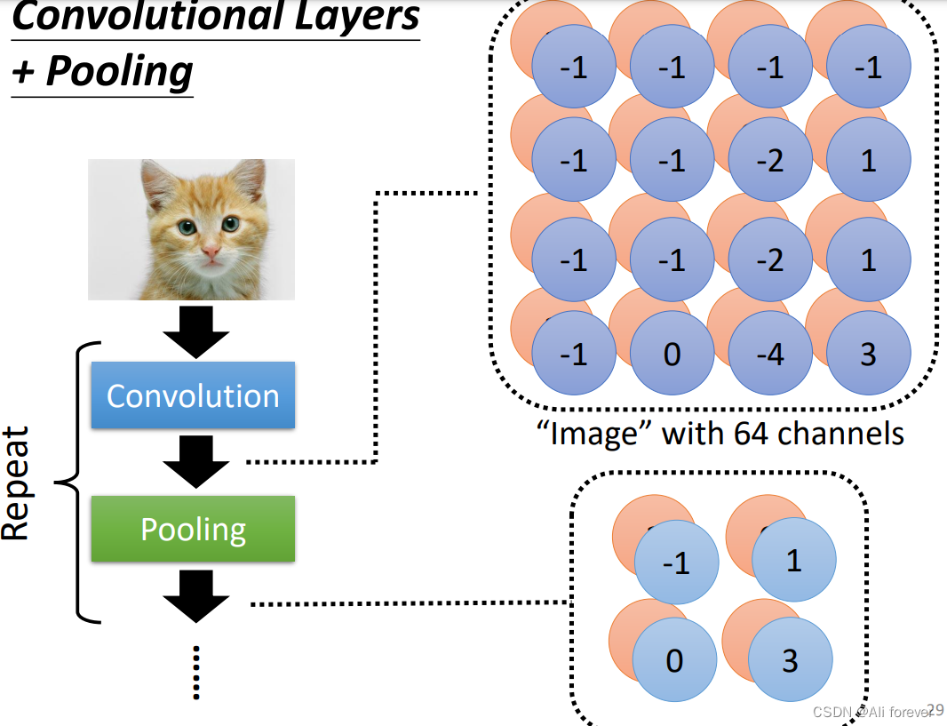
Pooling layer typically USES is to do a picture of a bigsubsampling(下采样),To set a convergence layer,Then in convergence range and one of the biggest value represents a part of this,但是channel不会改变.
但事实上,CNNNot to zoom in on picture,旋转等操作,The need to use image enhancement can be.
There are pooling layer formula for calculating the size of the output layer width:
W n e x t = ( W n o w − F ) S + 1 W_{next} =\frac{(W_{now}-F)}{S}+1 Wnext=S(Wnow−F)+1
其中S是步长,F是池化层的大小
4.全连接层
在卷积层的最后,We usually set a full connection layer,The convolution layer into full connection.The weight of the connection layer is a huge matrix,除了某些特定块(感受野),其余部分都是零;而在非 0 部分中,Most elements are equal(权值共享)
四、ICS(Internal Covariate shift)
1.ICS是什么?
深度神经网络涉及到很多层的叠加,而每一层的参数更新会导致上层的输入数据分布发生变化,层层叠加后,At the top of input distribution changes would obviously,For senior need to adapt to the underlying parameters update.This kind of problem we are calledICS问题.
2.ICS导致的问题
ICSCan lead to upper level network need to constantly adapt to the new input data distribution,降低学习速度.下层输入的变化可能趋向于变大或者变小,导致上层落入饱和区,使得学习过早停止.每层的更新都会影响到其它层,因此每层的参数更新策略需要尽可能的谨慎.
3.ICS的解决方法
解决ICSThe most direct ideas is to make the distribution of each layer are independent identically distributed
1.白化(whiting)
白化是对输入数据分布进行变换,进而达到以下两个目的:
- 使得输入特征分布具有相同的均值与方差,其中PCA白化保证了所有特征分布均值为0,方差为1;而ZCA白化则保证了所有特征分布均值为0,方差相同;
- 去除特征之间的相关性.
But an albino calculation cost is too high,Not suitable for use in large-scale computing
2.正则化(normalization)
NormalizationIs the average distribution of forced back to the for0方差为1的标准正态分布,使得激活输入值落在非线性函数对输入比较敏感的区域,这样输入的小变化就会导致损失函数较大的变化,避免梯度消失问题产生,加速收敛.
But if you are using a standardized,That is equivalent to the nonlinear activation function replace linear function,The establishment of a complex model that does not use,容易造成model bias.
3.Batch Normalization
Standardized on the single dimension of the input data,根据每一个batch计算均值与标准差,Because from the image is the calculation of longitudinal,Also known as the longitudinal standardization
五、Job code, a
1.题目要求

2.引入库
# Import necessary packages.
import numpy as np
import torch
import torch.nn as nn
import torchvision.transforms as transforms
from PIL import Image
# "ConcatDataset" and "Subset" are possibly useful when doing semi-supervised learning.
from torch.utils.data import ConcatDataset, DataLoader, Subset
from torchvision.datasets import ImageFolder
# This is for the progress bar.
from tqdm.auto import tqdm
torchvision包: torchvision是pytorch的一个图形库,它服务于PyTorch深度学习框架的,主要用来构建计算机视觉模型.以下是torchvision的构成:
torchvision.transforms:常用的图片变换,例如裁剪、旋转等
torchvision.datasets:Some data for the image functions and common data collection interface
torchvision.models: 包含常用的模型结构(含预训练模型),例如AlexNet、VGG、ResNet等
3.构造数据集
train_trm=transforms.Compose([transforms.Resize(128,128),transforms.ToTensor(),])
test_trm=transforms.Compose([transforms.Resize(128,128),transforms.ToTensor(),])

batch_size=128
train_set=ImageFolder("food-11/training/labeled", transform=train_tfm)
valid_set=ImageFolder("food-11/validation", transform=test_tfm)
unlabeled_set = ImageFolder("food-11/training/unlabeled",  transform=train_tfm)
test_set = ImageFolder("food-11/testing", transform=test_tfm)

train_loader=DataLoader(train_set,batch_size=batch_size,shuffle=True,num_work=0,pin_memory=True)
valid_loader=DataLoader(valid_set,batch_size=batch_size,shuffle=True,num_work=0,pin_memory=True)
test_loader=DataLoader(test_set,batch_size=batch_size,shuffle=False)
transforms.Compose:这个类的主要作用是串联多个图片变换的操作,Can see the contents of this class is a list of,Will traverse the list of operation.
transforms.Resize(128,128),transforms.ToTensor():前面是将PILThe dimension of the image changes,And then finally willPILChange images to aTensor向量.
torchvision.datasets.ImageFolder(root, transform=None, target_transform=None, loader=, is_valid_file=None):是一个容器,
root:图片存储的根目录,即各类别文件夹所在目录的上一级目录.
transform:In the pretreatment of image manipulation functions,原始图片作为输入,返回一个转换后的图片,
target_transform:对图片类别进行预处理的操作,输入为 target,输出对其的转换. 如果不传该参数,即对 target 不做任何转换,返回的顺序索引 0,1, 2…
4.CNN模型构造
After the deal with the data set in,We will build ourCNN模型,We can see that with the help ofnn.BatchNorm2d解决ICS问题
class Classifier(nn.Module):
    def __init__(self):
        super(Classifier, self).__init__()
        # The arguments for commonly used modules:
        # torch.nn.Conv2d(in_channels, out_channels, kernel_size, stride, padding)
        # torch.nn.MaxPool2d(kernel_size, stride, padding)

        # input image size: [3, 128, 128]
        self.cnn_layers = nn.Sequential(
            nn.Conv2d(3, 64, 3, 1, 1),
            nn.BatchNorm2d(64),
            nn.ReLU(),
            nn.MaxPool2d(2, 2, 0),

            nn.Conv2d(64, 128, 3, 1, 1),
            nn.BatchNorm2d(128),
            nn.ReLU(),
            nn.MaxPool2d(2, 2, 0),

            nn.Conv2d(128, 256, 3, 1, 1),
            nn.BatchNorm2d(256),
            nn.ReLU(),
            nn.MaxPool2d(4, 4, 0),
        )
        print()
        self.fc_layers = nn.Sequential(
            nn.Linear(256 * 8 * 8, 256),
            nn.ReLU(),
            nn.Linear(256, 256),
            nn.ReLU(),
            nn.Linear(256, 11)
        )

    def forward(self, x):
        # input (x): [batch_size, 3, 128, 128]
        # output: [batch_size, 11]

        # Extract features by convolutional layers.
        x = self.cnn_layers(x)

        # The extracted feature map must be flatten before going to fully-connected layers.
        x = x.flatten(1)

        # The features are transformed by fully-connected layers to obtain the final logits.
        x = self.fc_layers(x)
        return x
5.参数准备
# "cuda" only when GPUs are available.
device = "cuda" if torch.cuda.is_available() else "cpu"

# Initialize a model, and put it on the device specified.
model = Classifier().to(device)
model.device = device

# For the classification task, we use cross-entropy as the measurement of performance.
criterion = nn.CrossEntropyLoss()

# Initialize optimizer, you may fine-tune some hyperparameters such as learning rate on your own.
optimizer = torch.optim.Adam(model.parameters(), lr=0.0003, weight_decay=1e-5)

# The number of training epochs.
n_epochs = 80
6.训练模型
for epoch in range(n_epochs):
# ---------- Training ----------
# Make sure the model is in train mode before training.
model.train()
# These are used to record information in training.
train_loss = []
train_accs = []
# Iterate the training set by batches.
for batch in tqdm(train_loader):
# A batch consists of image data and corresponding labels.
imgs, labels = batch
# Forward the data. (Make sure data and model are on the same device.)
logits = model(imgs.to(device))
# Calculate the cross-entropy loss.
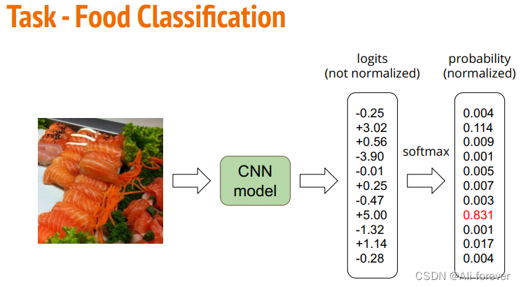
# We don't need to apply softmax before computing cross-entropy as it is done automatically.
loss = criterion(logits, labels.to(device))
# Gradients stored in the parameters in the previous step should be cleared out first.
optimizer.zero_grad()
# Compute the gradients for parameters.
loss.backward()
# Clip the gradient norms for stable training.
grad_norm = nn.utils.clip_grad_norm_(model.parameters(), max_norm=10)
# Update the parameters with computed gradients.
optimizer.step()
# Compute the accuracy for current batch.
acc = (logits.argmax(dim=-1) == labels.to(device)).float().mean()
# Record the loss and accuracy.
train_loss.append(loss.item())
train_accs.append(acc)
# The average loss and accuracy of the training set is the average of the recorded values.
train_loss = sum(train_loss) / len(train_loss)
train_acc = sum(train_accs) / len(train_accs)
# Print the information.
print(f"[ Train | {
epoch + 1:03d}/{
n_epochs:03d} ] loss = {
train_loss:.5f}, acc = {
train_acc:.5f}")
# ---------- Validation ----------
# Make sure the model is in eval mode so that some modules like dropout are disabled and work normally.
model.eval()
# These are used to record information in validation.
valid_loss = []
valid_accs = []
# Iterate the validation set by batches.
for batch in tqdm(valid_loader):
# A batch consists of image data and corresponding labels.
imgs, labels = batch
# We don't need gradient in validation.
# Using torch.no_grad() accelerates the forward process.
with torch.no_grad():
logits = model(imgs.to(device))
# We can still compute the loss (but not the gradient).
loss = criterion(logits, labels.to(device))
# Compute the accuracy for current batch.
acc = (logits.argmax(dim=-1) == labels.to(device)).float().mean()
# Record the loss and accuracy.
valid_loss.append(loss.item())
valid_accs.append(acc)
# The average loss and accuracy for entire validation set is the average of the recorded values.
valid_loss = sum(valid_loss) / len(valid_loss)
valid_acc = sum(valid_accs) / len(valid_accs)
# Print the information.
print(f"[ Valid | {
epoch + 1:03d}/{
n_epochs:03d} ] loss = {
valid_loss:.5f}, acc = {
valid_acc:.5f}")
7.测试数据
# Some modules like Dropout or BatchNorm affect if the model is in training mode.
model.eval()

# Initialize a list to store the predictions.
predictions = []

# Iterate the testing set by batches.
for batch in tqdm(test_loader):
    # A batch consists of image data and corresponding labels.
    # But here the variable "labels" is useless since we do not have the ground-truth.
    # If printing out the labels, you will find that it is always 0.
    # This is because the wrapper (DatasetFolder) returns images and labels for each batch,
    # so we have to create fake labels to make it work normally.
    imgs, labels = batch

    # We don't need gradient in testing, and we don't even have labels to compute loss.
    # Using torch.no_grad() accelerates the forward process.
    with torch.no_grad():
        logits = model(imgs.to(device))

    # Take the class with greatest logit as prediction and record it.
    predictions.extend(logits.argmax(dim=-1).cpu().numpy().tolist())
# Save predictions into the file.
with open("predict.csv", "w") as f:

    # The first row must be "Id, Category"
    f.write("Id,Category\n")

    # For the rest of the rows, each image id corresponds to a predicted class.
    for i, pred in  enumerate(predictions):
         f.write(f"{
      i},{
      pred}\n")
总结
本文介绍了CNN卷积神经网络,希望大家能从中获取到想要的东西,下面附上一张思维导图帮助记忆.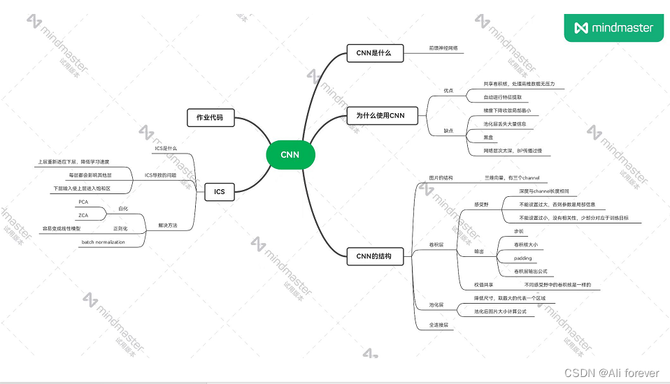
边栏推荐
- C# 四舍五入 MidpointRounding.AwayFromZero
- [LeetCode] Find the sum of the numbers from the root node to the leaf node
- 墨西哥大众VW Mexico常见的几种label
- Nacos源码分析专题(五)-Nacos小结
- Shell编程--awk
- 月薪35K,靠八股文就能做到的事,你居然不知道
- 实操|风控模型中常用的这三种预测方法与多分类场景的实现
- 彩色袜子题
- OpenCV图像处理学习四,像素的读写操作和图像反差函数操作
- ImportError: Unable to import required dependencies: numpy
猜你喜欢

Sikuli's Automated Testing Technology Based on Pattern Recognition

Premint工具,作为普通人我们需要了解哪些内容?
Nacos源码分析专题(五)-Nacos小结

OpenCV图像处理学习一,加载显示修改保存图像相关函数
odoo公用变量或数组的使用
Problems and solutions related to Chinese character set in file operations in ABAP

Maya制作赛博朋克机器人模型

C# rounding MidpointRounding.AwayFromZero

Initial attempt at UI traversal

万字总结:分布式系统的38个知识点
随机推荐
Unity3D创建道路插件EasyRoads的使用
【LeetCode】求根节点到叶节点数字之和
阿里云OSS文件上传
Experimental support for decorators may change in future releases.Set the "experimentalDecorators" option in "tsconfig" or "jsconfig" to remove this warning
51单片机驱动HMI串口屏,串口屏的下载方式
卷积神经网络识别验证码
彩色袜子题
16. 最接近的三数之和
Problems and solutions related to Chinese character set in file operations in ABAP
Shader Graph learns various special effects cases
SonarQube升级记录:7.8->7.9->8.9
多线程之享元模式和final原理
Nacos源码分析专题(五)-Nacos小结
Open3D 中点细分(网格细分)
Not, even the volume of the king to write code in the company are copying and pasting it reasonable?
免费文档翻译软件电脑版软件
网络爬虫错误
【web渗透】SSRF漏洞超详细讲解
[QNX Hypervisor 2.2用户手册]10.14 smmu
【SSRF漏洞】实战演示 超详细讲解