当前位置:网站首页>2.1 - Gradient Descent
2.1 - Gradient Descent
2022-08-11 07:51:00 【A big boa constrictor 6666】
文章目录
Return to that section in the previous chapter,We discussed the process of how to find a best model,That is, to find a set of parametersθ,让这个loss函数越小越好:
θ ∗ = a r g m i n θ L ( θ ) θ^{*}=arg\underset{θ}{min}L(θ) θ∗=argθminL(θ)
当θ有两个参数 { θ 1 , θ 2 } \{\theta _{1},\theta _{2}\} { θ1,θ2}时,A set of starting points is randomly selected θ 0 = [ θ 1 0 θ 2 0 ] \theta ^{0}=\begin{bmatrix} \theta _{1}^{0}\\ \theta _{2}^{0} \end{bmatrix} θ0=[θ10θ20],上标0Represents the initial set of parameters,下标1,2Represents are the first and second parameters in this set of parameters.
接下来计算 { θ 1 , θ 2 } \{\theta _{1},\theta _{2}\} { θ1,θ2}their respective partial differentials:
[ θ 1 1 θ 2 1 ] = [ θ 1 0 θ 2 0 ] − η [ ∂ L ( θ 1 0 ) ∂ θ 1 ∂ L ( θ 2 0 ) ∂ θ 2 ] \begin{bmatrix} \theta _{1}^{1}\\ \theta _{2}^{1} \end{bmatrix}=\begin{bmatrix} \theta _{1}^{0}\\ \theta _{2}^{0} \end{bmatrix}-\eta \begin{bmatrix} \frac{\partial L(\theta _{1}^{0})}{\partial \theta _{1}}\\ \frac{\partial L(\theta _{2}^{0})}{\partial \theta _{2}} \end{bmatrix} [θ11θ21]=[θ10θ20]−η[∂θ1∂L(θ10)∂θ2∂L(θ20)]
[ θ 1 2 θ 2 2 ] = [ θ 1 1 θ 2 1 ] − η [ ∂ L ( θ 1 1 ) ∂ θ 1 ∂ L ( θ 2 1 ) ∂ θ 2 ] \begin{bmatrix} \theta _{1}^{2}\\ \theta _{2}^{2} \end{bmatrix}=\begin{bmatrix} \theta _{1}^{1}\\ \theta _{2}^{1} \end{bmatrix}-\eta \begin{bmatrix} \frac{\partial L(\theta _{1}^{1})}{\partial \theta _{1}}\\ \frac{\partial L(\theta _{2}^{1})}{\partial \theta _{2}} \end{bmatrix} [θ12θ22]=[θ11θ21]−η[∂θ1∂L(θ11)∂θ2∂L(θ21)]
对于 { θ 1 , θ 2 } \{\theta _{1},\theta _{2}\} { θ1,θ2}There is another way of writing the partial differential of : ▽ L ( θ ) \bigtriangledown L(\theta) ▽L(θ)Also called gradient(Gradient),represents a set of vectors(vector)
▽ L ( θ ) = [ ∂ L ( θ 1 ) ∂ θ 1 ∂ L ( θ 2 ) ∂ θ 2 ] \bigtriangledown L(\theta)=\begin{bmatrix} \frac{\partial L(\theta _{1})}{\partial \theta _{1}}\\ \frac{\partial L(\theta _{2})}{\partial \theta _{2}} \end{bmatrix} ▽L(θ)=[∂θ1∂L(θ1)∂θ2∂L(θ2)]
- θ 1 = θ 0 − η ▽ L ( θ 0 ) \theta ^1=\theta ^0-\eta\bigtriangledown L(\theta ^0) θ1=θ0−η▽L(θ0)
- θ 2 = θ 1 − η ▽ L ( θ 1 ) \theta ^2=\theta ^1-\eta\bigtriangledown L(\theta ^1) θ2=θ1−η▽L(θ1)
The figure below is gradient descent(Gradient Descent)的可视化过程:The red arrows represent the direction of the gradient,The blue arrows represent the direction of parameter update,两者是相反的.

一、调整学习率
- 当你有3and more than one parameter,There is no way to visualize gradient descent(Gradient Descent)的过程的.However, the learning rate can be visualized(learning rate)η和Losscurve between values.

1.1 自适应学习率(Adaptive Learning Rates)
- 在开始时,Since we are far from the optimal solution,Therefore, a larger learning rate can be used,Increase the pace of gradient descent.
- After a few rounds of training,We are now closer to the optimal solution,So reduce the learning rate,Decrease the pace of gradient descent,Avoid oscillating around the optimal solution.
- The simplest strategy is to let the learning rate vary over time,如: η t = η t + 1 \eta^t=\frac{\eta}{\sqrt{t+1}} ηt=t+1η
- But not all parameters are suitable for such a set of adjustment strategies
1.2 Adagrad
- Adagradis the root mean square of each parameter's learning rate divided by its previous derivative value(root mean square )
Let's take a look at ordinary gradient descent(Vanilla Gradient descent)和Adagrad之间的区别:
- Vanilla Gradient descent:
- Font metrics not found for font: .
- Adagrad: σ t \sigma ^t σt代表参数wThe root mean square of all previous differential values(root mean square )
- Font metrics not found for font: .
- 下面是AdagradThe specific derivation process and the final simplified writing method:


- There are some inconsistencies in the final simplified notation(Contradiction)之处:当梯度g越大时,We are expecting a bigger pace of decline,But the denominator of the formula is preventing us from doing so.

对于这个问题,There are two such explanations:
- 直观的解释(Intuitive Reason):In order to emphasize the contrast effect of a certain gradient(特别大或者特别小),We added the term denominator
更正式的解释:
- 对于一个参数:When the steps we step out are proportional to the magnitude of the differential,Then it may be the best pace.
- Compare different parameters(Comparison between different parameters):In order to truly reflect the distance between the location and the lowest point,We're not just proportional to the gradientga derivative of ,It is also inversely proportional to the gradientg的二次微分.
The figure below is an explanation of the denominator term in the formula to estimate the quadratic differential:When sampling enough points,梯度gThe squared sum of , and then the square root can be approximately equal to the gradientg的二次微分


二、随机梯度下降(Stochastic Gradient Descent)
- Stochastic gradient descent is much faster than normal gradient descent:
- This is because for stochastic gradient descent,It will look at each oneexample的loss值,相当于走了20步


三、特征缩放(Feature Scaling)
- 将x1和x2Two different feature distributions are scaled to the same scale:
- 如右图,The point of this is to make it easier for us to do gradient descent,更加有效率.Because the starting point after feature scaling starts no matter where,The direction of gradient descent is always pointing to the lowest point.


- Z分数归一化(Z-Score Normalization)
- ZScore normalization is a common way to achieve feature scaling.It works by calculating each dimension(行)特征的均值mi和标准差σi,Then convert each value of the feature matrix x i r x_i^r xirAll minus the meanmi并除以标准差σi,这样更新后的 x i r x_i^r xirare all in0~1之间了.

四、数学推导
- 泰勒级数(Taylor Series):
- 设h(x)is an arbitrary functionx=x0Differentiable nearby,那么h(x)可以写成下面这样

- 多变量泰勒级数(Multivariable Taylor Series):
- According to the definition of Taylor series,If the red circle in the picture on the right is small enough,Then you can put it in the red circlelossThe function is simplified using Taylor series
- 简化之后,It becomes a search within the red circle θ 1 , θ 2 \theta_1,\theta_2 θ1,θ2使得lossproblem with the smallest value
- when the derivation reaches the last step,It becomes the formula we did gradient descent before,But the premise of the establishment of the formula is the radius of the red circler要足够小,由于学习率 η \eta η是和r成正比的,So the learning rate cannot be too large,Theoretically, it takes infinite hours for the formula to hold,But in the actual operation process as long as it is small enough.
- The above derivation process we use is the first-order form of Taylor series,When considering the quadratic,三次,even multiple times,Our requirements for the red circle are not so great,Theoretically, the learning rate can also be adjusted higher.But this is rarely done in deep learning,This is because the huge amount of computation that comes with it is unbearable.


五、梯度下降的限制(More Limitation of Gradient Descent)
- In the process of doing gradient descent,Actually looking for itloss函数微分为0的地方,However, the differential is0is not necessarily a local optimal solution,It could also be a saddle point in the graph.
- Also in the actual solution process,We're not looking for differentials to really do0的点,But when the differential is less than a certain number(如10的-6次方)的点,In fact, this point may still be a relatively high place,It is still far from the local optimal solution to be found.
- We will continue to discuss this issue in the next chapter

边栏推荐
- 1096 big beautiful numbers (15 points)
- Unity程序员如何提升自己的能力
- Redis source code: how to view the Redis source code, the order of viewing the Redis source code, the sequence of the source code from the external data structure of Redis to the internal data structu
- NTT的Another Me技术助力创造歌舞伎演员中村狮童的数字孪生体,将在 “Cho Kabuki 2022 Powered by NTT”舞台剧中首次亮相
- 接入网、承载网、核心网是什么,交换机路由器是什么、这个和网络的协议有什么关系呢?
- 【软件测试】(北京)字节跳动科技有限公司终面HR面试题
- 为什么我使用C#操作MySQL进行中文查询失败
- 接口测试的基础流程和用例设计方法你知道吗?
- 2022年中国软饮料市场洞察
- How Unity programmers can improve their abilities
猜你喜欢

【Pytorch】nn.PixelShuffle
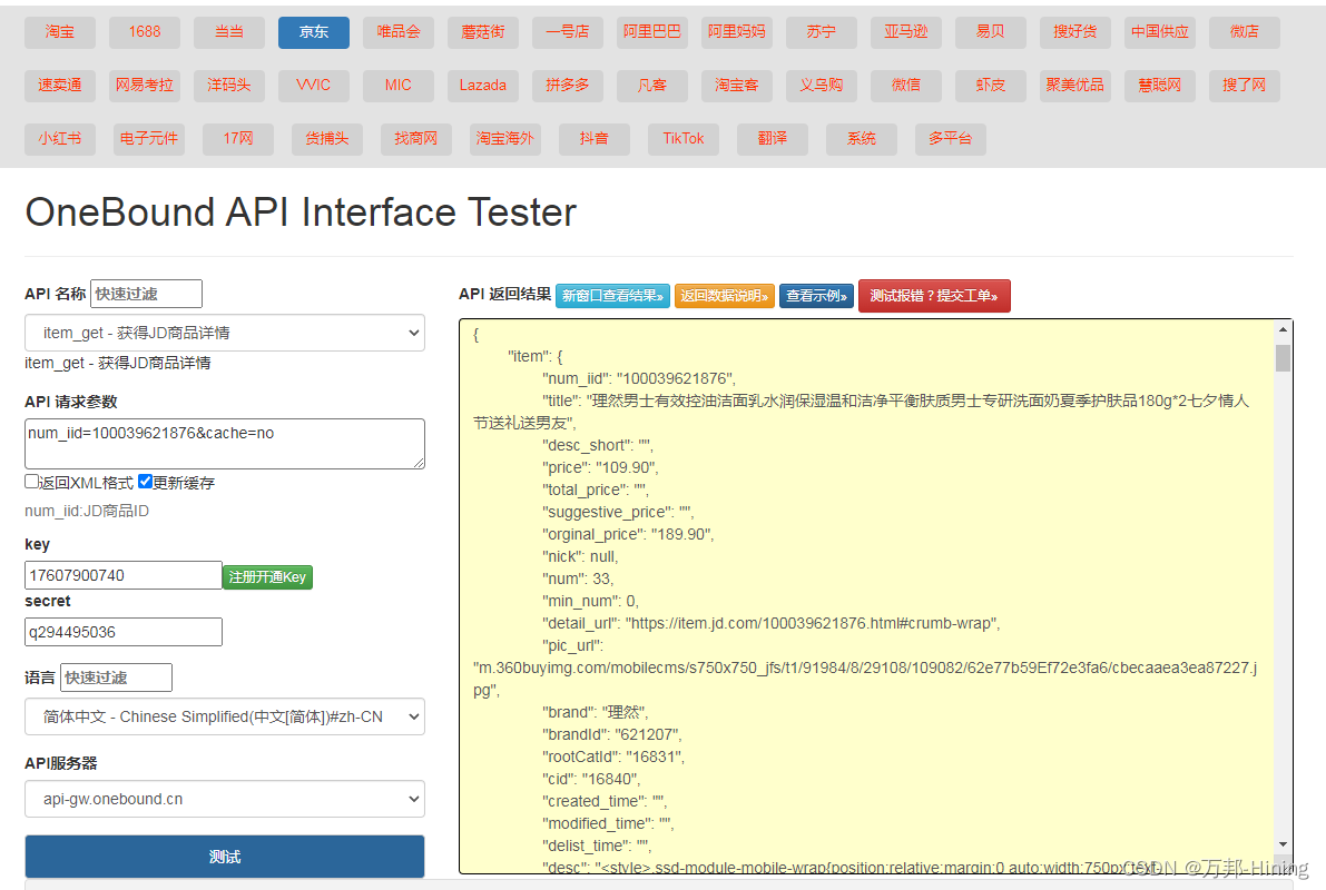
Strongly recommend an easy-to-use API interface
1101 B是A的多少倍 (15 分)
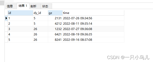
查找最新人员工资和上上次人员工资的变动情况

linux 安装mysql服务报错

测试用例很难?有手就行

年薪40W测试工程师成长之路,你在哪个阶段?

1003 I want to pass (20 points)
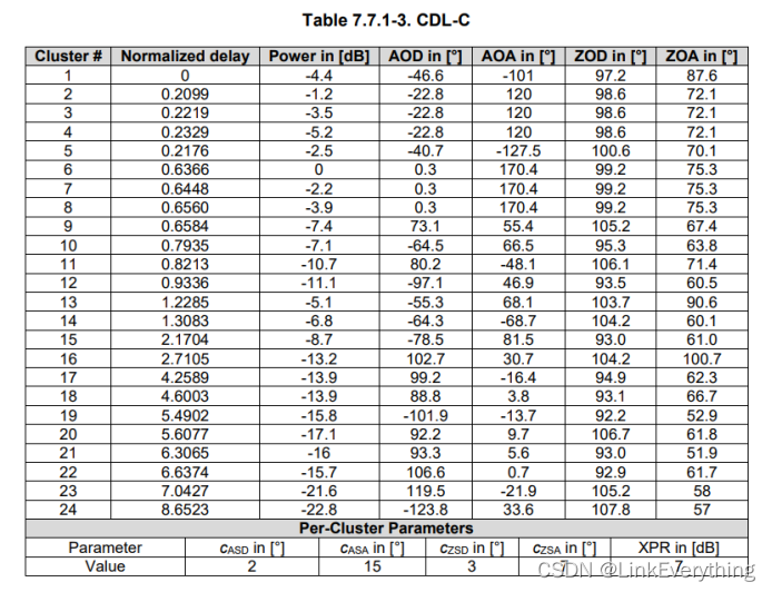
3GPP LTE/NR信道模型

【latex异常和错误】Missing $ inserted.<inserted text>You can‘t use \spacefactor in math mode.输出文本要注意特殊字符的转义
随机推荐
【LeetCode】链表题解汇总
从苹果、SpaceX等高科技企业的产品发布会看企业产品战略和敏捷开发的关系
prometheus学习4Grafana监控mysql&blackbox了解
golang fork 进程的三种方式
1091 N-Defensive Number (15 points)
1081 检查密码 (15 分)
TF通过feature与label生成(特征,标签)集合,tf.data.Dataset.from_tensor_slices
1106 2019数列 (15 分)
4.1 - Support Vector Machines
linux 安装mysql服务报错
2022-08-09 第四小组 修身课 学习笔记(every day)
Unity游戏排行榜的制作与优化
【推荐系统】:协同过滤和基于内容过滤概述
2022年中国软饮料市场洞察
MindManager2022全新正式免费思维导图更新
3.1-分类-概率生成模型
TF中的四则运算
MySQL使用GROUP BY 分组查询时,SELECT 查询字段包含非分组字段
Strongly recommend an easy-to-use API interface
关于#sql#的问题:怎么将下面的数据按逗号分隔成多行,以列的形式展示出来