Machine learning II: logistic regression classification based on Iris data set

Step1: Library function import

#  Basic function library 
import numpy as np 
import pandas as pd

#  Drawing function library 
import matplotlib.pyplot as plt
import seaborn as sns

Iris data set （iris） It includes 5 A variable , among 4 Characteristic variables ,1 A target classification variable . share 150 Samples , The target variable is the category of flowers , They all belong to three subgenera of iris , Namely Iris iris (Iris-setosa), Color fleur-de-lis (Iris-versicolor) and Iris Virginia (Iris-virginica). It contains four characteristics of three Iris species , Namely Calyx length (cm)、 Calyx width (cm)、 Petal length (cm)、 Petal width (cm), These morphological features have been used in the past to identify species .

Variable	describe
sepal length	Calyx length (cm)
sepal width	Calyx width (cm)
petal length	Petal length (cm)
petal width	Petal width (cm)
target	Three subgenera of iris ,‘setosa’(0), ‘versicolor’(1), ‘virginica’(2)

Step2: data fetch / load

#  utilize  sklearn  The built-in  iris  Data is loaded as data , And make use of Pandas Turn into DataFrame Format 
from sklearn.datasets import load_iris
data = load_iris() #  Get the data features 
iris_target = data.target #  Get the tag corresponding to the data 
iris_features = pd.DataFrame(data=data.data, columns=data.feature_names) #  utilize Pandas Turn into DataFrame Format 

Step3: Simple view of data information

##  utilize .info() View the overall information of the data 
iris_features.info()

<class ‘pandas.core.frame.DataFrame’>
RangeIndex: 150 entries, 0 to 149
Data columns (total 4 columns):
Column Non-Null Count Dtype

---

0 sepal length (cm) 150 non-null float64
1 sepal width (cm) 150 non-null float64
2 petal length (cm) 150 non-null float64
3 petal width (cm) 150 non-null float64
dtypes: float64(4)
memory usage: 4.8 KB

##  Do a simple data view , We can use  .head()  Head .tail() The tail 
iris_features.head()

iris_features.tail()

##  The corresponding category label is , among 0,1,2 Represent the 'setosa', 'versicolor', 'virginica' Three different types of flowers .
iris_target

array([0, 0, 0, 0, 0, 0, 0, 0, 0, 0, 0, 0, 0, 0, 0, 0, 0, 0, 0, 0, 0, 0,
0, 0, 0, 0, 0, 0, 0, 0, 0, 0, 0, 0, 0, 0, 0, 0, 0, 0, 0, 0, 0, 0,
0, 0, 0, 0, 0, 0, 1, 1, 1, 1, 1, 1, 1, 1, 1, 1, 1, 1, 1, 1, 1, 1,
1, 1, 1, 1, 1, 1, 1, 1, 1, 1, 1, 1, 1, 1, 1, 1, 1, 1, 1, 1, 1, 1,
1, 1, 1, 1, 1, 1, 1, 1, 1, 1, 1, 1, 2, 2, 2, 2, 2, 2, 2, 2, 2, 2,
2, 2, 2, 2, 2, 2, 2, 2, 2, 2, 2, 2, 2, 2, 2, 2, 2, 2, 2, 2, 2, 2,
2, 2, 2, 2, 2, 2, 2, 2, 2, 2, 2, 2, 2, 2, 2, 2, 2, 2])

##  utilize value_counts Function to see the number of each category 
pd.Series(iris_target).value_counts()

2 50
1 50
0 50
dtype: int64

##  Some statistical description of the features 
iris_features.describe()

From the statistical description, we can see the variation range of different numerical characteristics .

Step4: Visual description

#  Combine tag and feature information 
iris_all = iris_features.copy() ## Make a light copy , Prevent modification of original data 
iris_all['target'] = iris_target

#  Scatter visualization of feature and tag combination 
sns.pairplot(data=iris_all,diag_kind='hist', hue= 'target')
plt.show()

Draw a box diagram ：

• Five elements of box diagram ： .
• 1、 Median ： That is, the half quantile . So the calculation method is to put a set of data （ The median here , Especially an ordered sequence arranged from large to small ） Divide equally into two parts , Take the middle number . If the original sequence length n Is odd , So the median is (n+1)/2; If the original sequence length n It's even , So the median is n/2,n/2+1, The value of the median is equal to the arithmetic mean of the numbers at these two positions .
• 2、 Upper quartile Q1： emphasize , How to find the quartile , Is to divide the sequence equally into four parts . At present, the specific calculation has (n+1)/4 And (n-1)/4 Two kinds of , In general use (n+1)/4.
  for example ： An ordered sequence test = c(1,2,3,4,5,6,7,8), adopt summary(test) To get test The median of this sequence , Upper quartile , Lower quartile and arithmetic mean . First, the sequence length n=8,(1+n)/4=2.25, Explain that the upper quartile is in the 2.25 Number of positions , So the first 2.25 The number is the second number 0.25+ The third number 0.75, namely 20.25+3*0.75=0.5+2.25=2.75.
• 3、 Lower quartile Q3： The calculation method of the position of the lower quartile is the same as above , nothing but (1+n)/43=6.75, This is a place between the sixth position and the seventh position . The corresponding specific value is 0.756+0.25*7=6.25.
• 4、 Internal limit ： above T The extreme distance to which a line segment extends , yes Q3+1.5IQR( among ,IQR=Q3-Q1) And the maximum value after excluding outliers , Below T The extreme distance to which a line segment extends , yes Q1-1.5IQR And the minimum value after excluding outliers, whichever is the maximum .
  （1,6,2,7,4,2,3,3,8,25,30）
  IQR=Q3-Q1=7.5-2.5=5
  Upper and inner limits =Q3+1.5IQR=7.5+1.55=15, And eliminate two abnormal addresses 30,25 The maximum after 8, Take the minimum of both , So the upper and inner limits are 8
  Lower internal limit =Q1-1.5IQR=2.5-1.55=-5, And eliminate two abnormal addresses 30,25 The minimum after 1, Take the maximum of both , So the lower limit is 1
• 5、 External limit ： The calculation method of outer limit and inner limit is the same , The only difference is with ： above T The extreme distance to which a line segment extends , yes Q3+3IQR( among ,IQR=Q3-Q1) And the maximum value after excluding outliers , Below T The extreme distance to which a line segment extends , yes Q1-3IQR And the minimum value after excluding outliers, whichever is the maximum .

for col in iris_features.columns:
    sns.boxplot(x='target', y=col, saturation=0.5,palette='pastel', data=iris_all)
    plt.title(col)
    plt.show()

The biggest advantage of box chart is : Not affected by outliers , It can describe the discrete distribution of data in a relatively stable way .

Using box graph, we can also get the distribution differences of different categories on different features .

#  Select the first three features to draw a three-dimensional scatter map 
from mpl_toolkits.mplot3d import Axes3D

fig = plt.figure(figsize=(10,8))
ax = fig.add_subplot(111, projection='3d')

iris_all_class0 = iris_all[iris_all['target']==0].values
iris_all_class1 = iris_all[iris_all['target']==1].values
iris_all_class2 = iris_all[iris_all['target']==2].values
# 'setosa'(0), 'versicolor'(1), 'virginica'(2)
ax.scatter(iris_all_class0[:,0], iris_all_class0[:,1], iris_all_class0[:,2],label='setosa')
ax.scatter(iris_all_class1[:,0], iris_all_class1[:,1], iris_all_class1[:,2],label='versicolor')
ax.scatter(iris_all_class2[:,0], iris_all_class2[:,1], iris_all_class2[:,2],label='virginica')
plt.legend()

plt.show()

Step5: utilize Logistic regression model In the second category Train and predict

##  In order to correctly evaluate the model performance , Divide the data into training set and test set , And train the model on the training set , Verify model performance on a test set .
from sklearn.model_selection import train_test_split

##  Select the category as 0 and 1 The sample of  （ Excluding categories of 2 The sample of ）
iris_features_part = iris_features.iloc[:100]
iris_target_part = iris_target[:100]

##  The test set size is 20%, 80%/20% branch 
x_train, x_test, y_train, y_test = train_test_split(iris_features_part, iris_target_part, test_size = 0.2, random_state = 2020)

##  from sklearn The logistic regression model is introduced into the model 
from sklearn.linear_model import LogisticRegression

##  Definition   Logistic regression model  
clf = LogisticRegression(random_state=0, solver='lbfgs')

#  Train the logistic regression model on the training set 
clf.fit(x_train, y_train)

LogisticRegression(C=1.0, class_weight=None, dual=False, fit_intercept=True,
intercept_scaling=1, l1_ratio=None, max_iter=100,
multi_class=‘auto’, n_jobs=None, penalty=‘l2’,
random_state=0, solver=‘lbfgs’, tol=0.0001, verbose=0,
warm_start=False)

##  Look at the corresponding w
print('the weight of Logistic Regression:',clf.coef_)

##  Look at the corresponding w0
print('the intercept(w0) of Logistic Regression:',clf.intercept_)

the weight of Logistic Regression: [[ 0.45181973 -0.81743611 2.14470304 0.89838607]]
the intercept(w0) of Logistic Regression: [-6.53367714]

##  In the training set and test set distribution, using the trained model to predict 
train_predict = clf.predict(x_train)
test_predict = clf.predict(x_test)

from sklearn import metrics

##  utilize accuracy（ Accuracy ）【 The proportion of the number of correctly predicted samples to the total number of predicted samples 】 Evaluate the effect of the model 
print('The accuracy of the Logistic Regression is:',metrics.accuracy_score(y_train,train_predict))
print('The accuracy of the Logistic Regression is:',metrics.accuracy_score(y_test,test_predict))

##  Look at the confusion matrix  ( Statistical matrix of various situations of predicted value and real value )
confusion_matrix_result = metrics.confusion_matrix(test_predict,y_test)
print('The confusion matrix result:\n',confusion_matrix_result)

#  The results are visualized using thermal maps 
plt.figure(figsize=(8, 6))
sns.heatmap(confusion_matrix_result, annot=True, cmap='Blues')
plt.xlabel('Predicted labels')
plt.ylabel('True labels')
plt.show()

The accuracy of the Logistic Regression is: 1.0
The accuracy of the Logistic Regression is: 1.0
The confusion matrix result:
[[ 9 0]
[ 0 11]]

It can be found that the accuracy is 1, It means that all samples are correctly predicted .

Step6: utilize Logistic regression model In three categories ( Many classification ) On Train and predict

##  The test set size is 20%, 80%/20% branch 
x_train, x_test, y_train, y_test = train_test_split(iris_features, iris_target, test_size = 0.2, random_state = 2020)

##  Definition   Logistic regression model  
clf = LogisticRegression(random_state=0, solver='lbfgs')

#  Train the logistic regression model on the training set 
clf.fit(x_train, y_train)

LogisticRegression(C=1.0, class_weight=None, dual=False, fit_intercept=True,
intercept_scaling=1, l1_ratio=None, max_iter=100,
multi_class=‘auto’, n_jobs=None, penalty=‘l2’,
random_state=0, solver=‘lbfgs’, tol=0.0001, verbose=0,
warm_start=False)

##  Look at the corresponding w
print('the weight of Logistic Regression:\n',clf.coef_)

##  Look at the corresponding w0
print('the intercept(w0) of Logistic Regression:\n',clf.intercept_)

##  Because this is 3 classification , So here we get the parameters of three logistic regression models , The three logistic regression can be combined to realize the three classification .

the weight of Logistic Regression:
[[-0.45928925 0.83069886 -2.26606531 -0.9974398 ]
[ 0.33117319 -0.72863423 -0.06841147 -0.9871103 ]
[ 0.12811606 -0.10206463 2.33447679 1.9845501 ]]
the intercept(w0) of Logistic Regression:
[ 9.43880677 3.93047364 -13.36928041]

##  In the training set and test set distribution, using the trained model to predict 
train_predict = clf.predict(x_train)
test_predict = clf.predict(x_test)

##  Since the logistic regression model is a probabilistic prediction model （ Previously described  p = p(y=1|x,\theta)）, All we can do with  predict_proba  Function predicts its probability 
train_predict_proba = clf.predict_proba(x_train)
test_predict_proba = clf.predict_proba(x_test)

print('The test predict Probability of each class:\n',test_predict_proba)
##  The first column represents the prediction of 0 The probability of a class , The second column represents the prediction of 1 The probability of a class , The third column represents the prediction of 2 The probability of a class .

##  utilize accuracy（ Accuracy ）【 The proportion of the number of correctly predicted samples to the total number of predicted samples 】 Evaluate the effect of the model 
print('The accuracy of the Logistic Regression is:',metrics.accuracy_score(y_train,train_predict))
print('The accuracy of the Logistic Regression is:',metrics.accuracy_score(y_test,test_predict))

The test predict Probability of each class:
[[1.03461734e-05 2.33279475e-02 9.76661706e-01]
[9.69926591e-01 3.00732875e-02 1.21676996e-07]
[2.09992547e-02 8.69156617e-01 1.09844128e-01]
[3.61934870e-03 7.91979966e-01 2.04400685e-01]
[7.90943202e-03 8.00605300e-01 1.91485268e-01]
[7.30034960e-04 6.60508053e-01 3.38761912e-01]
[1.68614209e-04 1.86322045e-01 8.13509341e-01]
[1.06915332e-01 8.90815532e-01 2.26913667e-03]
[9.46928070e-01 5.30707294e-02 1.20016057e-06]
[9.62346385e-01 3.76532233e-02 3.91897289e-07]
[1.19533384e-04 1.38823468e-01 8.61056998e-01]
[8.78881883e-03 6.97207361e-01 2.94003820e-01]
[9.73938143e-01 2.60617346e-02 1.22613836e-07]
[1.78434056e-03 4.79518177e-01 5.18697482e-01]
[5.56924342e-04 2.46776841e-01 7.52666235e-01]
[9.83549842e-01 1.64500670e-02 9.13617258e-08]
[1.65201477e-02 9.54672749e-01 2.88071038e-02]
[8.99853708e-03 7.82707576e-01 2.08293887e-01]
[2.98015025e-05 5.45900066e-02 9.45380192e-01]
[9.35695863e-01 6.43039513e-02 1.85301359e-07]
[9.80621190e-01 1.93787400e-02 7.00125246e-08]
[1.68478815e-04 3.30167226e-01 6.69664295e-01]
[3.54046163e-03 4.02267805e-01 5.94191734e-01]
[9.70617284e-01 2.93824740e-02 2.42443967e-07]
[2.56895205e-04 1.54631583e-01 8.45111522e-01]
[3.48668490e-02 9.11966141e-01 5.31670105e-02]
[1.47218847e-02 6.84038115e-01 3.01240001e-01]
[9.46510447e-04 4.28641987e-01 5.70411503e-01]
[9.64848137e-01 3.51516748e-02 1.87917880e-07]
[9.70436779e-01 2.95624025e-02 8.18591606e-07]]
The accuracy of the Logistic Regression is: 0.9833333333333333
The accuracy of the Logistic Regression is: 0.8666666666666667

##  Look at the confusion matrix 
confusion_matrix_result = metrics.confusion_matrix(test_predict,y_test)
print('The confusion matrix result:\n',confusion_matrix_result)

#  The results are visualized using thermal maps 
plt.figure(figsize=(8, 6))
sns.heatmap(confusion_matrix_result, annot=True, cmap='Blues')
plt.xlabel('Predicted labels')
plt.ylabel('True labels')
plt.show()

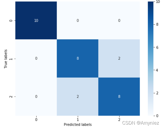
Through the results we can find , The prediction accuracy of the three classification results has declined , Its accuracy on the test set is :$86.67\%$, This is because ’versicolor’（1） and ‘virginica’（2） The characteristics of these two categories , We can also see from the visualization that , The boundary of its characteristics is fuzzy （ The boundary categories are mixed , There is no clear distinction between borders ）, There are some mistakes in these two kinds of predictions .