当前位置:网站首页>【论文阅读】RAL 2022: Receding Moving Object Segmentation in 3D LiDAR Data Using Sparse 4D Convolutions
【论文阅读】RAL 2022: Receding Moving Object Segmentation in 3D LiDAR Data Using Sparse 4D Convolutions
2022-08-08 16:27:00 【Kin__Zhang】
参考与前言
Status: Finished
Type: RAL
Year: 2022
论文链接:https://www.ipb.uni-bonn.de/wp-content/papercite-data/pdf/mersch2022ral.pdf
代码链接:https://github.com/PRBonn/4DMOS
1. Motivation
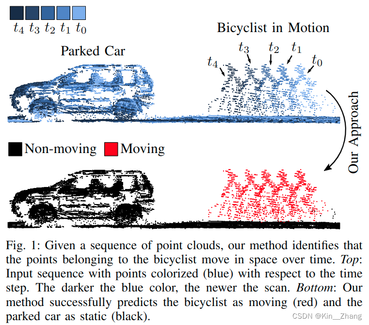
在自动驾驶导航中 dynamics obstacle 对于轨迹规划很重要,所以如何识别动态障碍物是一个比较重要的问题
问题场景
现有方法:
- 使用BEV角度的LiDAR Image进入2D Conv CNN进行提取 temporal info,通常这种 projection 2D表示 是从3D里聚类 比如 kNN
- 在建图过程中,根据聚类和tracking进行检测 运动点云
以上方法都是offline 需要时间内所有的LiDAR;其他方法也有对比两相邻帧点云的
本文方法主要focus on object that in a limited time horizon
Contribution
可以通过short sequence的LiDAR信息预测moving objects
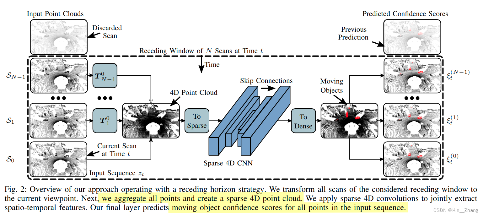
exploit sparse 4D Conv 从LiDAR点云中提取时空特征。方法输出:每个点云是否是动态物体的confidence scores,设计了一个一定大小的滑动窗口,超过一定删除旧frame
- 比现有方法 更精准的识别动态物体
- 对于unseen的场景有好的泛化性
- 通过在线新的观测输入,改进已知结果
2. Method
前提假设:已知所有帧帧之间的translation matrix T \boldsymbol T T,point点表示 p i = [ x i , y i , z i , t i ] ⊤ \boldsymbol{p}_{i}=\left[x_{i}, y_{i}, z_{i}, t_i\right]^{\top} pi=[xi,yi,zi,ti]⊤ ,因为室外的点云较为稀疏,所以将4D点云到sparse voxel grid,时间和空间的resolution分别为 Δ t , Δ s \Delta t, \Delta s Δt,Δs
使用一个稀疏的tensor保存voxel grid的indices和相关features
2.1 框架
2.2 Sparse 4D
稀疏4D卷积使用的是:Minkowski engine, NVIDIA做的一款开源的稀疏张量的自动微分库,比起dense conv,主要是为了加速
使用的是修改后的 MinkUNet14 [8],a sparse equivalent of a residual bottleneck architecture with strided sparse convolutions for downsampling the feature maps and strided sparse transpose convolutions for upsampling
不同于4D分割使用RGB作为input features,本文首先初始化voxels,被至少一个点占据时constant feature是0.5;因此我们的输入仅保存有点占据的voxel
这样部署到新环境下,不需要再考虑coordinates distribution或是通过intensity value对输入数据进行标准化了
下面为源码抽取的代码 进行的数据处理和sparse:
quantization = self.quantization.type_as(past_point_clouds[0])
past_point_clouds = [
   torch.div(point_cloud, quantization) for point_cloud in past_point_clouds
]
features = [
    0.5 * torch.ones(len(point_cloud), 1).type_as(point_cloud)
    for point_cloud in past_point_clouds
]

coords, features = ME.utils.sparse_collate(past_point_clouds, features)
tensor_field = ME.TensorField(
    features=features, coordinates=coords.type_as(features)
)

sparse_tensor = tensor_field.sparse()

predicted_sparse_tensor = self.MinkUNet(sparse_tensor)
2.3 Receding Horizon
经过上面的步骤后,网络会输出每个输入序列点上的confidence score。在实际运行网络时 inference time,避免重复输出同一帧的,一般是选择将输入数据进行切分固定;本文则是采取receding horizon,接收新的 就扔旧的 如上框架图
2.4 Binary Bayes Filter
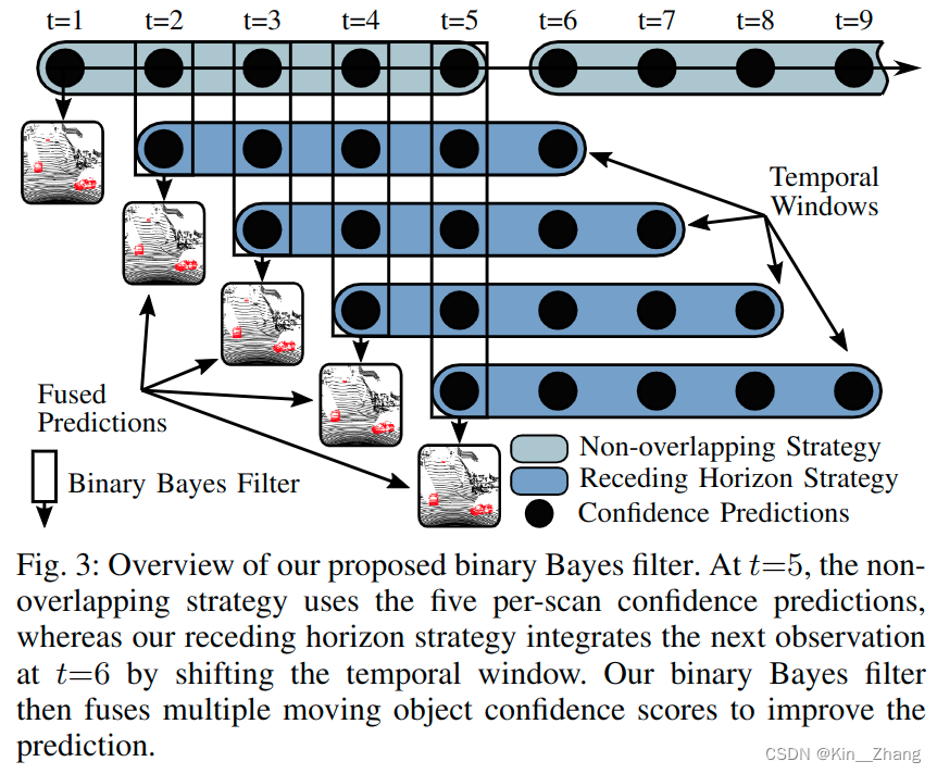
本文的方法是直接预测的N个scan的输入,输出一个结果,receding horizon则可以通过接收新的一帧,re-estimate 前N-1的scans;对于多次预测结果我们使用binary bayes filter进行融合
贝叶斯融合层可以减少因为传感器噪音或被遮挡住时,输出错误的 false positive和negatives的数量
我们想预测的是 所有点在整个时间内对 motion state m ( j ) m^{(j)} m(j) 的联合概率:
p ( m ( j ) ∣ z 0 : t ( j ) ) = ∏ i p ( m i ( j ) ∣ z 0 : t ( j ) ) (2) p\left(m^{(j)} \mid z_{0: t}^{(j)}\right)=\prod_{i} p\left(m_{i}^{(j)} \mid z_{0: t}^{(j)}\right) \tag{2} p(m(j)∣z0:t(j))=i∏p(mi(j)∣z0:t(j))(2)
m ( j ) ∈ { 0 , 1 } m^{(j)} \in \{0,1\} m(j)∈{ 0,1} 表示 点 p i ∈ S j p_i \in S_j pi∈Sj的状态是否是moving, S j S_j Sj为第j次扫描的LiDAR输入,后面的公式为了简洁点 把j就省去了哈
我们使用bayes’ rule在公式2上,然后follow standard derivation of the recursive binary bayes filter [36],下面的l为 l ( x ) = log p ( x ) 1 − p ( x ) l(x)=\log \frac{p(x)}{1-p(x)} l(x)=log1−p(x)p(x) 通常在占用栅格地图上使用,如下进行更新:
l ( m i ∣ z 0 : t ) = { l ( m i ∣ z 0 : t − 1 ) + l ( m i ∣ z t ) − l ( m i ) , if t ∈ T l ( m i ∣ z 0 : t − 1 ) , otherwise (3) l\left(m_{i} \mid z_{0: t}\right)= \begin{cases}l\left(m_{i} \mid z_{0: t-1}\right)+l\left(m_{i} \mid z_{t}\right)-l\left(m_{i}\right), & \text { if } t \in \mathcal{T} \\ l\left(m_{i} \mid z_{0: t-1}\right), & \text { otherwise }\end{cases} \tag{3} l(mi∣z0:t)={ l(mi∣z0:t−1)+l(mi∣zt)−l(mi),l(mi∣z0:t−1), if t∈T otherwise (3)
prior probability p 0 ∈ ( 0 , 1 ) p_0 \in (0,1) p0∈(0,1) provides a measure of the innovation introduced by a new prediction. 这个值同样决定了how much 在单帧内的一个 predicted moving point 对于最后的prediction造成的影响
为网络输出的scores对应到上面moving的概率
ξ t , i = p ( m i = 1 ∣ z t ) (4) \xi_{t, i}=p\left(m_{i}=1 \mid z_{t}\right) \tag{4} ξt,i=p(mi=1∣zt)(4)
则log-odds confidence的指数为:
l ( m i ∣ z t ) = log ξ t , i 1 − ξ t , i (5) l\left(m_{i} \mid z_{t}\right)=\log \frac{\xi_{t, i}}{1-\xi_{t, i}} \tag{5} l(mi∣zt)=log1−ξt,iξt,i(5)
然后经过公式3等,取回概率 p ( x ) = log l ( x ) 1 + l ( x ) p(x)=\log \frac{l(x)}{1+l(x)} p(x)=log1+l(x)l(x) 如果这个confidence score大于0.5 则认为这个点是移动的 反之是静止
代码对应
# Bayesian Fusion
elif strategy == "bayes":
    for pred_idx, confidences in tqdm(dict_confidences.items(), desc="Scans"):
        confidence = np.load(confidences[0])
        log_odds = prob_to_log_odds(confidence)
        for conf in confidences[1:]:
            confidence = np.load(conf)
            log_odds += prob_to_log_odds(confidence)
            log_odds -= prob_to_log_odds(prior * np.ones_like(confidence))
        final_confidence = log_odds_to_prob(log_odds)
        pred_labels = to_label(final_confidence, semantic_config)
        pred_labels.tofile(pred_path + "/" + pred_idx.split(".")[0] + ".label")
verify_predictions(seq, pred_path, semantic_config)

def to_label(confidence, semantic_config):
    pred_labels = np.ones_like(confidence)
    pred_labels[confidence > 0.5] = 2
    pred_labels = to_original_labels(pred_labels, semantic_config)
    pred_labels = pred_labels.reshape((-1)).astype(np.int32)
    return pred_labels
3. 实验及结果
消融实验做的挺多,很仔细的,metric主要是针对运动物体所在的点的IoU
I o U M O S = T P T P + F P + F N \mathrm{IoU}_{\mathrm{MOS}}=\frac{\mathrm{TP}}{\mathrm{TP}+\mathrm{FP}+\mathrm{FN}} IoUMOS=TP+FP+FNTP

上面提到的 p 0 p_0 p0的赋值会产生IoU值的不同
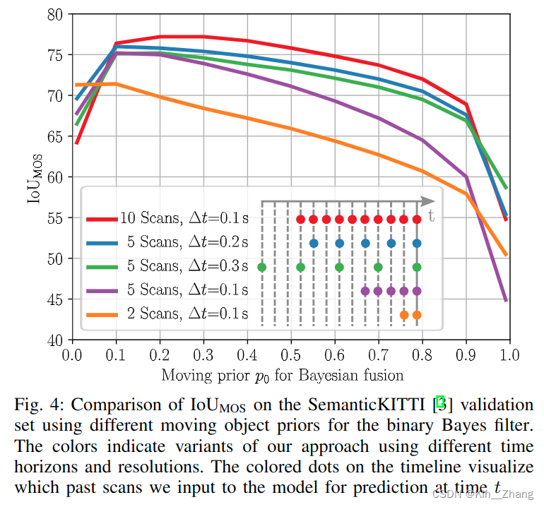

其中表三的 Δ t \Delta t Δt 为不同的时间分辨率下
对于运行的时间也有讨论,Python运行,整个网络如果是10次scans的话平均是0.078s,5次scans的话0.047s 在NVIDIA RTX A5000;bayes filter分别需要0.008s 0.004s对于10和5次
4. Conclusion
重复一下方法和contribution部分:
使用receding horizon对输入序列进行动态障碍物的预测,同时结合了binary bayes filter在时间维度上对预测结果进行融合,增加鲁棒性
未来工作可以在于里程计上的优化,因为在本文讨论时,里程计设置为已知状态。
赠人点赞 手有余香 ;正向回馈 才能更好开放记录 hhh
边栏推荐
- web automation headless mode
- leetcode 155. Min Stack最小栈(中等)
- 本博客目录及版权申明
- Take you to play with the "Super Cup" ECS features and experiment on the pit [HUAWEI CLOUD is simple and far]
- Spark cluster environment construction
- 毕设-基于SSM学生考试系统
- spark集群环境搭建
- 我分析30w条数据后发现,西安新房公摊最低的竟是这里?
- Taro小程序跨端开发入门实战
- ggplot2可视化水平箱图并使用fct_reorder排序数据、使用na.rm处理缺失值(reorder boxplot with fct_reorder)、按照箱图的中位数从大到小排序水平箱图
猜你喜欢
Kubernetes资源编排系列之四: CRD+Operator篇
【MATLAB项目实战】基于Morlet小波变换的滚动轴承故障特征提取研究
![[Unity entry plan] Use the double blood bar method to control the blood loss speed of the damage area](/img/d3/13bff820963988678f3a3361abc3aa.png)
[Unity entry plan] Use the double blood bar method to control the blood loss speed of the damage area

The origin and creation of Smobiler's complex controls

Share these new Blender plugins that designers must not miss in 2022

GHOST工具访问数据库
Grid 布局介绍
groovy基础学习
Flutter的实现原理初探

成员变量和局部变量的区别?
随机推荐
在通达信开户安全不呢
函数节流与函数防抖
9. cuBLAS Development Guide Chinese Version--Configuration of Atomic Mode in cuBLAS
pytorch安装过程中出现torch.cuda.isavailable()=False问题
api的封装
高数_证明_基本初等函数的导数公式
ggplot2可视化水平箱图并使用fct_reorder排序数据、使用na.rm处理缺失值(reorder boxplot with fct_reorder)、按照箱图的中位数从大到小排序水平箱图
‘xxxx‘ is declared but its value is never read.Vetur(6133)
[Online interviewer] How to achieve deduplication and idempotency
The situation of the solution of the equation system and the correlation transformation of the vector group
开源项目管理解决方案Leantime
用于视觉语言导航的自监督三维语义表示学习
鹏城杯部分WP
淘宝API常用接口列表与申请方式
Share these new Blender plugins that designers must not miss in 2022
web automation headless mode
它们不一样!透析【观察者模式】和【发布订阅模式】
GHOST tool to access the database
Taro小程序跨端开发入门实战
带你玩转“超大杯”ECS特性及实验踩坑【华为云至简致远】