The first 1 Chapter NumPy Basics

link

1.1 Generate NumPy Array

1.1.1 Create an array from existing data

Direct pair Python Basic data type of ( As listing 、 Tuples etc. ) Transform to generate ndarray:
（1） Convert the list to ndarray

import numpy as np
 
lst1 = [3.14, 2.17, 0, 1, 2]
nd1 =np.array(lst1)
print(nd1)
# [3.14 2.17 0.   1.   2.  ]
print(type(nd1))
# <class 'numpy.ndarray'>

（2） Nested lists can be converted into multidimensional lists ndarray

import numpy as np
 
lst2 = [[3.14, 2.17, 0, 1, 2], [1, 2, 3, 4, 5]]
nd2 =np.array(lst2)
print(nd2)
# [[3.14 2.17 0.   1.   2.  ]
#  [1.   2.   3.   4.   5.  ]]
print(type(nd2))
# <class 'numpy.ndarray'>

If you replace the list in the above example with tuples, it is also suitable .

1.1.2 utilize random Module generates an array

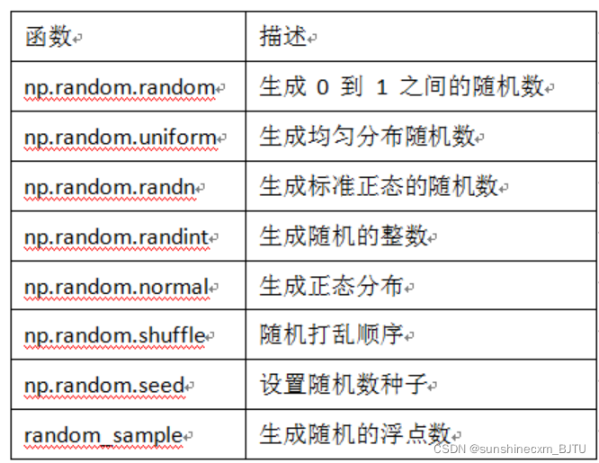
surface 1-1 np.random Module common functions

Let's take a look at the specific use of some functions :

import numpy as np
 
nd3 =np.random.random([3, 3])
print(nd3)
# [[0.43007219 0.87135582 0.45327073]
#  [0.7929617  0.06584697 0.82896613]
#  [0.62518386 0.70709239 0.75959122]]
print("nd3 The shape of is :",nd3.shape)
# nd3 The shape of is : (3, 3)

In order to generate the same data every time , You can specify a random seed , Use shuffle Function disrupts the generated random number .

import numpy as np
 
np.random.seed(123)
nd4 = np.random.randn(2,3)
print(nd4)
np.random.shuffle(nd4)
print(" After random disruption, the data :")
print(nd4)
print(type(nd4))

 Output results :
[[-1.0856306 0.99734545 0.2829785 ]
[-1.50629471 -0.57860025 1.65143654]]
 After random disruption, the data :
[[-1.50629471 -0.57860025 1.65143654]
[-1.0856306 0.99734545 0.2829785 ]]

1.1.3 Create a multidimensional array of specific shapes

Parameter initialization , Sometimes you need to generate some special matrices , If all are 0 or 1 An array or matrix of , Then we can use np.zeros、np.ones、np.diag To achieve , As shown in the table 1-2 Shown .
surface 1-2 NumPy Array creation function

Let's illustrate with a few examples :

import numpy as np
 
#  Generation is all  0  Of  3x3  matrix 
nd5 =np.zeros([3, 3])
# Generation and nd5 All in the same shape 0 matrix 
#np.zeros_like(nd5)
#  Generation is all  1  Of  3x3  matrix 
nd6 = np.ones([3, 3])
#  Generate  3  The unit matrix of order 
nd7 = np.eye(3)
#  Generate  3  Diagonal matrix of order 
nd8 = np.diag([1, 2, 3])
 
print(nd5)
# [[0. 0. 0.]
#  [0. 0. 0.]
#  [0. 0. 0.]]
print(nd6)
# [[1. 1. 1.]
#  [1. 1. 1.]
#  [1. 1. 1.]]
print(nd7)
# [[1. 0. 0.]
#  [0. 1. 0.]
#  [0. 0. 1.]]
print(nd8)
# [[1 0 0]
#  [0 2 0]
#  [0 0 3]]

Sometimes we may need to save the generated data temporarily , For future use .

import numpy as np
 
nd9 =np.random.random([5, 5])
np.savetxt(X=nd9, fname='./test1.txt')
nd10 = np.loadtxt('./test1.txt')
print(nd10)

 Output results :
[[0.41092437 0.5796943 0.13995076 0.40101756 0.62731701]
[0.32415089 0.24475928 0.69475518 0.5939024 0.63179202]
[0.44025718 0.08372648 0.71233018 0.42786349 0.2977805 ]
[0.49208478 0.74029639 0.35772892 0.41720995 0.65472131]
[0.37380143 0.23451288 0.98799529 0.76599595 0.77700444]]

1.1.4 utilize arange、linspace Function to generate an array

• arange yes numpy Functions in modules , The format for :

arange([start,] stop[,step,], dtype=None)

among start And stop Specified scope ,step Set the step size , Generate a ndarray,start The default is 0, step step It can be a decimal .Python There's a built-in function range The function is similar .

import numpy as np
 
print(np.arange(10))
# [0 1 2 3 4 5 6 7 8 9]
print(np.arange(0, 10))
# [0 1 2 3 4 5 6 7 8 9]
print(np.arange(1, 4, 0.5))
# [1.  1.5 2.  2.5 3.  3.5]
print(np.arange(9, -1, -1))
# [9 8 7 6 5 4 3 2 1 0]

• linspace It's also numpy Functions commonly used in modules , The format for :

np.linspace(start, stop, num=50, endpoint=True, retstep=False, dtype=None)

It can specify the data range and equal quantity according to the input , Automatically generate a linear bisection vector , among endpoint ( Including the end point ) The default is True, Divide the quantity equally num The default is 50. If you will retstep Set to True, Will return a step size ndarray.

import numpy as np
 
print(np.linspace(0, 1, 10))
#[0.         0.11111111 0.22222222 0.33333333 0.44444444 0.55555556
# 0.66666667 0.77777778 0.88888889 1.        ]

Worth mentioning , It's not as we expected , Generate 0.1, 0.2, … 1.0 So the step size is 0.1 Of ndarray, This is because linspace It must contain the data starting point and ending point , Then the step size is (1-0) / 9 = 0.11111111. If you need to generate 0.1, 0.2, … 1.0 Data like this , Just start the data 0 It is amended as follows 0.1 that will do .
In addition to the above arange and linspace,NumPy It also provides logspace function , This function is used in the same way as linspace Use the same way , Readers might as well try it by themselves .

1.2 Get elements

In the previous section, we introduced generating ndarray Several ways to , After the data is generated , How to read the data we need ？ In this section, we introduce several common methods .

import numpy as np
np.random.seed(2019)
nd11 = np.random.random([10])
# Get the data of the specified location , For the first 4 Elements 
nd11[3]
# Intercept a piece of data 
nd11[3:6]
# Intercept fixed interval data 
nd11[1:6:2]
# Access in reverse order 
nd11[::-2]
# Intercept the data in a region of a multidimensional array 
nd12=np.arange(25).reshape([5,5])
nd12[1:3,1:3]
# Intercept a multidimensional array , Data whose value is within a range 
nd12[(nd12>3)&(nd12<10)]
# Intercept from multidimensional array , Specified row , For example, read page 2,3 That's ok 
nd12[[1,2]]  # or nd12[1:3,:]
## Intercept from multidimensional array , Specified column , For example, read page 2,3 Column 
nd12[:,1:3]

Let's further illustrate... By means of graphics , Pictured 1-1 Shown , On the left is the expression , On the right is the element obtained by the expression . Pay attention to different boundaries , Represent different expressions .

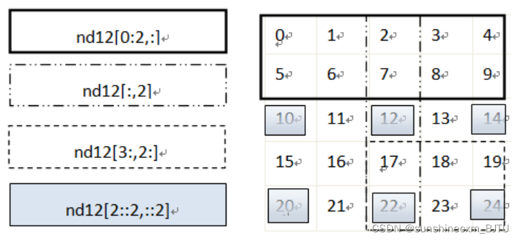
chart 1-1 Gets the elements in a multidimensional array

Get some elements in the array, except by specifying the index label , You can also use some functions to implement , Such as through random.choice Function can randomly extract data from a specified sample .

import numpy as np
from numpy import random as nr
 
a=np.arange(1,25,dtype=float)
c1=nr.choice(a,size=(3,4))  #size Specifies the shape of the output array 
c2=nr.choice(a,size=(3,4),replace=False)  #replace Default is True, You can repeatedly extract .
# In the following formula, the parameter p Specify the extraction probability corresponding to each element , The default is that each element has the same probability of being extracted .
c3=nr.choice(a,size=(3,4),p=a / np.sum(a))
print(" Random and repeatable extraction ")
print(c1)
print(" Random but not repeated extraction ")
print(c2)
print(" Random but according to institutional probability ")
print(c3)

 Print the results ：
 Random and repeatable extraction 
[[ 7. 22. 19. 21.]
[ 7. 5. 5. 5.]
[ 7. 9. 22. 12.]]
 Random but not repeated extraction 
[[ 21. 9. 15. 4.]
[ 23. 2. 3. 7.]
[ 13. 5. 6. 1.]]
 Random but according to institutional probability 
[[ 15. 19. 24. 8.]
[ 5. 22. 5. 14.]
[ 3. 22. 13. 17.]]

1.3 NumPy The arithmetic operation of

In machine learning and deep learning , Involving a large number of array or matrix operations , In this section, we focus on two common operations . One is to multiply the corresponding elements , Also known as unary multiplication (element-wise product), The operator is np.multiply(), or *. The other is dot product or inner product elements , The operator is np.dot().

1.3.1 Multiply the corresponding elements

Multiply the corresponding elements （element-wise product） Is the product of the corresponding elements in two matrices .np.multiply The function is used to multiply the corresponding elements of an array or matrix , The output is consistent with the size of the multiplied array or matrix , The format is as follows :

numpy.multiply(x1, x2, /, out=None, *, where=True,casting='same_kind', order='K', dtype=None, subok=True[, signature, extobj])

among x1,x2 The multiplication of corresponding elements between follows the broadcast rules ,NumPy The broadcasting rules of this chapter 7 This section will introduce . Let's use some examples to further illustrate .

A = np.array([[1, 2], [-1, 4]])
B = np.array([[2, 0], [3, 4]])
A*B
## give the result as follows ：
array([[ 2,  0],
       [-3, 16]])
# Or another representation 
np.multiply(A,B)
# The result of the calculation is also 
array([[ 2,  0],
       [-3, 16]])

matrix A and B The corresponding elements of are multiplied by , Use pictures 1-2 Intuitively expressed as ：

chart 1-2 Schematic diagram of corresponding element multiplication

NumPy An array can not only be multiplied by the corresponding elements of the array , It can also be combined with a single value （ Or scalar ） Carry out operations . Operation time ,NumPy Array each element and scalar operation , Broadcast mechanism will be used （1.7 This section details ）.

print(A*2.0)
print(A/2.0)

[[ 2. 4.]
[-2. 8.]]
[[ 0.5 1. ]
[-0.5 2. ]]

thus , By extension , After the array passes some activation functions , The output is consistent with the input shape .

X=np.random.rand(2,3)
def softmoid(x):
    return 1/(1+np.exp(-x))
def relu(x):
    return np.maximum(0,x)
def softmax(x):
    return np.exp(x)/np.sum(np.exp(x))
 
print(" Input parameters X The shape of the ：",X.shape)
print(" Activation function softmoid Shape of the output ：",softmoid(X).shape)
print(" Activation function relu Shape of the output ：",relu(X).shape)
print(" Activation function softmax Shape of the output ：",softmax(X).shape)

 Input parameters X The shape of the ： (2, 3)
 Activation function softmoid Shape of the output ： (2, 3)
 Activation function relu Shape of the output ： (2, 3)
 Activation function softmax Shape of the output ： (2, 3)

1.3.2 Dot product operations

Dot product operations （dot product） Also known as inner product , stay NumPy use np.dot Express , Its general format is ：

numpy.dot(a, b, out=None)

The following is illustrated by an example dot Specific use and precautions .

X1=np.array([[1,2],[3,4]])
X2=np.array([[5,6,7],[8,9,10]])
X3=np.dot(X1,X2)
print(X3)

[[21 24 27]
[47 54 61]]

The above calculation , Use pictures 1-3 Can be expressed as ：

chart 1-3 Schematic diagram of dot product of matrix , The number of elements in the corresponding dimension should be consistent

Pictured 1-3 Shown , matrix X1 And matrices X2 Perform dot product operation , among X1 and X2 Corresponding dimension （ namely X1 Of the 2 Three dimensions and X2 Of the 1 Dimensions ） The number of elements must be consistent , Besides , matrix X3 The shape of is determined by the matrix X1 The number of rows and matrix X2 The number of columns of .

1.4 Array deformation

In the tasks of machine learning and deep learning , It is usually necessary to feed the processed data to the model in a format acceptable to the model , Then the model passes through a series of operations , Finally, a processing result is returned . However , Because different models accept different input formats , A series of deformations and operations are often needed first , So as to process the data into a format that meets the requirements of the model . The most common is the operation of matrix or array , We often encounter the need to merge multiple vectors or matrices in a certain axis direction , Or need to flatten （ For example, in convolution or cyclic neural networks , Before the full connection layer , You need to flatten the matrix ）. Several common data deformation methods are introduced below .

1.4.1 Change the shape of the array

Modifying the shape of the specified array is NumPy One of the most common operations in , There are many common methods , surface 1-3 Lists some common functions .

surface 1-3 NumPy Some functions that change the shape of vectors in

Let's take a look at some examples :
（1）reshape

import numpy as np
 
arr =np.arange(10)
print(arr)
#  Vector  arr  The dimension is transformed into 2 That's ok 5 Column 
print(arr.reshape(2, 5))
#  When specifying dimensions, you can only specify the number of rows or columns ,  Other use  -1  Instead of 
print(arr.reshape(5, -1))
print(arr.reshape(-1, 5))

 Output results :
[0 1 2 3 4 5 6 7 8 9]

[[0 1 2 3 4]
[5 6 7 8 9]]

[[0 1]
[2 3]
[4 5]
[6 7]
[8 9]]

[[0 1 2 3 4]
[5 6 7 8 9]]

It is worth noting that ,reshape The function supports specifying only the number of rows or columns , The remaining settings are -1 that will do . The specified number of rows or columns must be divisible （ Such as 10 Can not be 3 to be divisible by ）, For example, if the above code is modified to arr.reshape(3,-1) Error will be reported .
（2）resize

import numpy as np
 
arr =np.arange(10)
print(arr)
#  Vector  arr  The dimension is transformed into 2 That's ok 5 Column 
arr.resize(2, 5)
print(arr)

 Output results :
[0 1 2 3 4 5 6 7 8 9]

[[0 1 2 3 4]
[5 6 7 8 9]]

（3）.T

import numpy as np
 
arr =np.arange(12).reshape(3,4)
#  vector  arr  by 3 That's ok 4 Column 
print(arr)
#  Vector  arr  Transpose to 4 That's ok 3 Column 
print(arr.T)

 Output results :
[[ 0 1 2 3]
[ 4 5 6 7]
[ 8 9 10 11]]
[[ 0 4 8]
[ 1 5 9]
[ 2 6 10]
[ 3 7 11]]

（4）ravel

import numpy as np
 
arr =np.arange(6).reshape(2, -1)
print(arr)
#  Priority by column , Flattening 
print(" Priority by column , Flattening ")
print(arr.ravel('F'))
#  Priority by line , Flattening 
print(" Priority by line , Flattening ")
print(arr.ravel())

 Output results :
[[0 1 2]
[3 4 5]]
 Priority by column , Flattening 
[0 3 1 4 2 5]
 Priority by line , Flattening 
[0 1 2 3 4 5]

（5）flatten
Convert a matrix into a vector , This requirement often occurs between convolutional network and full connection layer .

import numpy as np
a =np.floor(10*np.random.random((3,4)))
print(a)
print(a.flatten())

 Output results :
[[4. 0. 8. 5.]
[1. 0. 4. 8.]
[8. 2. 3. 7.]]

[4. 0. 8. 5. 1. 0. 4. 8. 8. 2. 3. 7.]

（6）squeeze
This is an important function for dimensionality reduction , Include... In the matrix 1 Remove the dimension of . stay Pytorch There is another opposite operation in ,torch.unsqueeze This will be introduced later .

import numpy as np
 
arr =np.arange(3).reshape(3, 1)
print(arr.shape)  #(3,1)
print(arr.squeeze().shape)  #(3,)
arr1 =np.arange(6).reshape(3,1,2,1)
print(arr1.shape) #(3, 1, 2, 1)
print(arr1.squeeze().shape) #(3, 2)

（7）transpose
Axis exchange of high-dimensional matrix , This is often used in deep learning , For example, the picture represents the color RGB The order , Change it to GBR The order of .

import numpy as np
 
arr2 = np.arange(24).reshape(2,3,4)
print(arr2.shape)  #(2, 3, 4)
print(arr2.transpose(1,2,0).shape)  #(3, 4, 2)

1.4.2 Merge array

Merging arrays is also one of the most common operations , surface 1-4 Lists the common methods for array or vector merging .
surface 1-4 NumPy Array merging method

[ explain ]
①append、concatnate as well as stack There is one. axis Parameters , Used to control whether array merging is by row or column .
② about append and concatnate, The array to be merged must have the same number of rows or columns ( Meet one ).
③stack、hstack、dstack The arrays to be merged must have the same shape ( shape).
Let's choose some common functions to explain .
（1）append
Merge one-dimensional arrays

import numpy as np
 
a =np.array([1, 2, 3])
b = np.array([4, 5, 6])
c = np.append(a, b)
print(c) 
# [1 2 3 4 5 6]

Merge multidimensional arrays

import numpy as np
 
a =np.arange(4).reshape(2, 2)
b = np.arange(4).reshape(2, 2)
#  Merge by line 
c = np.append(a, b, axis=0)
print(' The result after merging by row ')
print(c)
print(' Data dimension after consolidation ', c.shape)
#  Merge by columns 
d = np.append(a, b, axis=1)
print(' The result after merging by column ')
print(d)
print(' Data dimension after consolidation ', d.shape)

 Output results :
 The result after merging by row 
[[0 1]
[2 3]
[0 1]
[2 3]]
 Data dimension after consolidation  (4, 2)

 The result after merging by column 
[[0 1 0 1]
[2 3 2 3]]
 Data dimension after consolidation  (2, 4)

（2）concatenate
Joins an array or matrix along a specified axis

import numpy as np
a =np.array([[1, 2], [3, 4]])
b = np.array([[5, 6]])
 
c = np.concatenate((a, b), axis=0)
print(c)
d = np.concatenate((a, b.T), axis=1)
print(d)

 Output results :
[[1 2]
[3 4]
[5 6]]
[[1 2 5]
[3 4 6]]

（3）stack
Stacks an array or matrix along a specified axis

import numpy as np
 
a =np.array([[1, 2], [3, 4]])
b = np.array([[5, 6], [7, 8]])
print(np.stack((a, b), axis=0))

 Output results :
[[[1 2]
[3 4]]

[[5 6]
[7 8]]]

1.5 Batch processing

In deep learning , Because the source data is relatively large , Therefore, batch processing is usually required . For example, the random gradient method using batch to calculate the gradient （SGD）, Is a typical application . The calculation of deep learning is generally complex , In addition, the amount of data is generally large , If you process the whole data at once , There are often resource bottlenecks . For more efficient calculation , Generally, the whole data set is divided into small batches . The other extreme of processing an entire dataset is processing one record at a time , This method is also unscientific , Processing one record at a time cannot give full play to GPU、NumPy Advantages of parallel processing . therefore , Batch processing is often used in practical use （mini-batch）.
How to split big data into multiple batches ？ The following steps can be taken ：
（1） Get the dataset
（2） Randomly scramble data
（3） Define batch size
（4） Batch dataset

Let's use an example to illustrate ：

import numpy as np
# Generate 10000 The shape is 2X3 Matrix 
data_train = np.random.randn(10000,2,3)
# This is a 3 D matrix , The first dimension is the number of samples , The last two are data shapes 
print(data_train.shape)
#(10000,2,3)
# Disrupt this 10000 Data 
np.random.shuffle(data_train)
# Define batch size 
batch_size=100
# Batch processing 
for i in range(0,len(data_train),batch_size):
    x_batch_sum=np.sum(data_train[i:i+batch_size])
    print(" The first {} batch , Sum of data of this batch :{}".format(i,x_batch_sum))

 Last 5 Row result ：
 The first 9500 batch , Sum of data of this batch :17.63702580438092
 The first 9600 batch , Sum of data of this batch :-1.360924607368387
 The first 9700 batch , Sum of data of this batch :-25.912226239266445
 The first 9800 batch , Sum of data of this batch :32.018136957835814
 The first 9900 batch , Sum of data of this batch :2.9002576614446935

【 explain 】
Batch from 0 Start , So the last batch is 9900.

1.6 The generic function

NumPy Two basic objects are provided , namely ndarray and ufunc object . We introduced ndarray, This section will cover that NumPy Another object general function of (ufunc),ufunc yes universal function Abbreviation , It's a function that can operate on every element of an array . many ufunc All functions use c Language level implementation , So they're very fast . Besides , Their ratio math The functions in the module are more flexible .math The input of the module is generally scalar , but NumPy The function can be a vector or a matrix , The use of vectors or matrices can avoid the use of circular statements , This is in machine learning 、 It is very important in deep learning . surface 1-5 by NumPy Several common functions .

surface 1-5 NumPy Several common general functions

（1）math And numpy Function performance comparison ：

import time
import math
import numpy as np
 
x = [i * 0.001 for i in np.arange(1000000)]
start = time.clock()
for i, t in enumerate(x):
    x[i] = math.sin(t)
print ("math.sin:", time.clock() - start )
 
x = [i * 0.001 for i in np.arange(1000000)]
x = np.array(x)
start = time.clock()
np.sin(x)
print ("numpy.sin:", time.clock() - start )

Print the results

math.sin: 0.5169950000000005
numpy.sin: 0.05381199999999886

thus it can be seen ,numpy.sin Than math.sin Get close 10 times .

（2） Comparison of loop and vector operations ：
Make full use of Python Of NumPy Built in functions in the library （built-in function）, Realize the vectorization of calculation , It can greatly improve the running speed .NumPy The built-in functions in the library use SIMD Instructions . The vectorization used below is much faster than using loops . If you use GPU, Its performance will be more powerful , however NumPy I won't support it GPU.Pytorch Support GPU, The first 5 Chapter will introduce Pytorch How to use GPU To speed up the algorithm .

import time
import numpy as np
 
x1 = np.random.rand(1000000)
x2 = np.random.rand(1000000)
## Use a loop to calculate the vector dot product 
tic = time.process_time()
dot = 0
for i in range(len(x1)):
    dot+= x1[i]*x2[i]
toc = time.process_time()
print ("dot = " + str(dot) + "\n for loop----- Computation time = " + str(1000*(toc - tic)) + "ms")
## Use numpy Find the dot product of a function 
tic = time.process_time()
dot = 0
dot = np.dot(x1,x2)
toc = time.process_time()

print ("dot = " + str(dot) + "\n verctor version---- Computation time = " + str(1000*(toc - tic)) + "ms")

Output results

dot = 250215.601995
for loop----- Computation time = 798.3389819999998ms
dot = 250215.601995
verctor version---- Computation time = 1.885051999999554ms

In terms of running results , Use for The running time of the loop is about the same as that of vector operation 400 times . therefore , Deep learning algorithm , Vectorization matrix operation is generally used .

1.7 Broadcast mechanism

NumPy Of Universal functions Array required in shape It's consistent , When an array is shape When it's not equal , The broadcast mechanism will be used . however , Adjust the array so that shape equally , Need to meet certain rules , Otherwise, it will be wrong . These rules can be summed up in the following four ：

（1） Let all input arrays go into it shape The longest array is the same ,shape The insufficient parts in the are all preceded by 1 A filling ;
Such as ：a：2x3x2 b：3x2, be b towards a par , stay b In front of the 1： Turn into ：1x3x2
（2） Output array's shape Is the input array shape Maximum on each axis of ;
（3） If an axis of the input array is the same length as the corresponding axis of the output array, or its length is 1 when , This array can be used to calculate , Otherwise mistakes ;
（4） When the length of an axis of the input array is 1 when , All operations along this axis use （ Or copy ） The first set of values on this axis .
Broadcast throughout NumPy Used to decide how to deal with arrays with different shapes ; Involving arithmetic operations, including (+,-,*,/…). These rules are very strict , But it's not intuitive , Let's further explain with graphics and code ：
Purpose ：A+B
among A by 4x1 matrix ,B Is a one-dimensional vector (3,)
To add , You need to do the following ：
（1） According to rules 1,B Need to keep up with , hold B Turn into （1,3）
（2） According to rules 2, The output result is the maximum value on each axis , That is, the output result should be （4,3） matrix
that A How to make use of （4,1） Turn into （4,3） matrix ？B How to make use of （1,3） Turn into （4,3） matrix ？
（3） According to rules 4, Use the first set of values on this axis （ It is important to distinguish which axis ）, replicate （ But in actual processing, it is not really copied , Otherwise, it will consume too much memory , Instead, other objects such as ogrid object , Grid processing ） that will do ,
The detailed processing is shown in the figure 1-4 Shown .

chart 1-4 NumPy Schematic diagram of broadcasting rules

Code implementation

import numpy as np
A = np.arange(0, 40,10).reshape(4, 1)
B = np.arange(0, 3)
print("A The shape of matrix :{},B The shape of matrix :{}".format(A.shape,B.shape))
C=A+B
print("C The shape of matrix :{}".format(C.shape))
print(C)

Running results

A The shape of matrix :(4, 1),B The shape of matrix :(3,)
C The shape of matrix :(4, 3)
[[ 0 1 2]
[10 11 12]
[20 21 22]
[30 31 32]]

1.8 Summary

This chapter mainly introduces NumPy Common operation modules , In particular, it involves the operation of the matrix , These operations are often used in subsequent programs .NumPy It's rich in content , Here are only some main contents , If you want to know more , You can log in NumPy Official website ：http://www.numpy.org/