当前位置:网站首页>使用神经网络进行医学影像识别分析
使用神经网络进行医学影像识别分析
2022-08-11 11:07:00 【格格巫 MMQ!!】
近年高速发展的人工智能技术应用到了各个垂直领域,比如把深度学习应用于各种医学诊断,效果显著甚至在某些方面甚至超过了人类专家。典型的 CV 最新技术已经应用于阿尔茨海默病的分类、肺癌检测、视网膜疾病检测等医学成像任务中。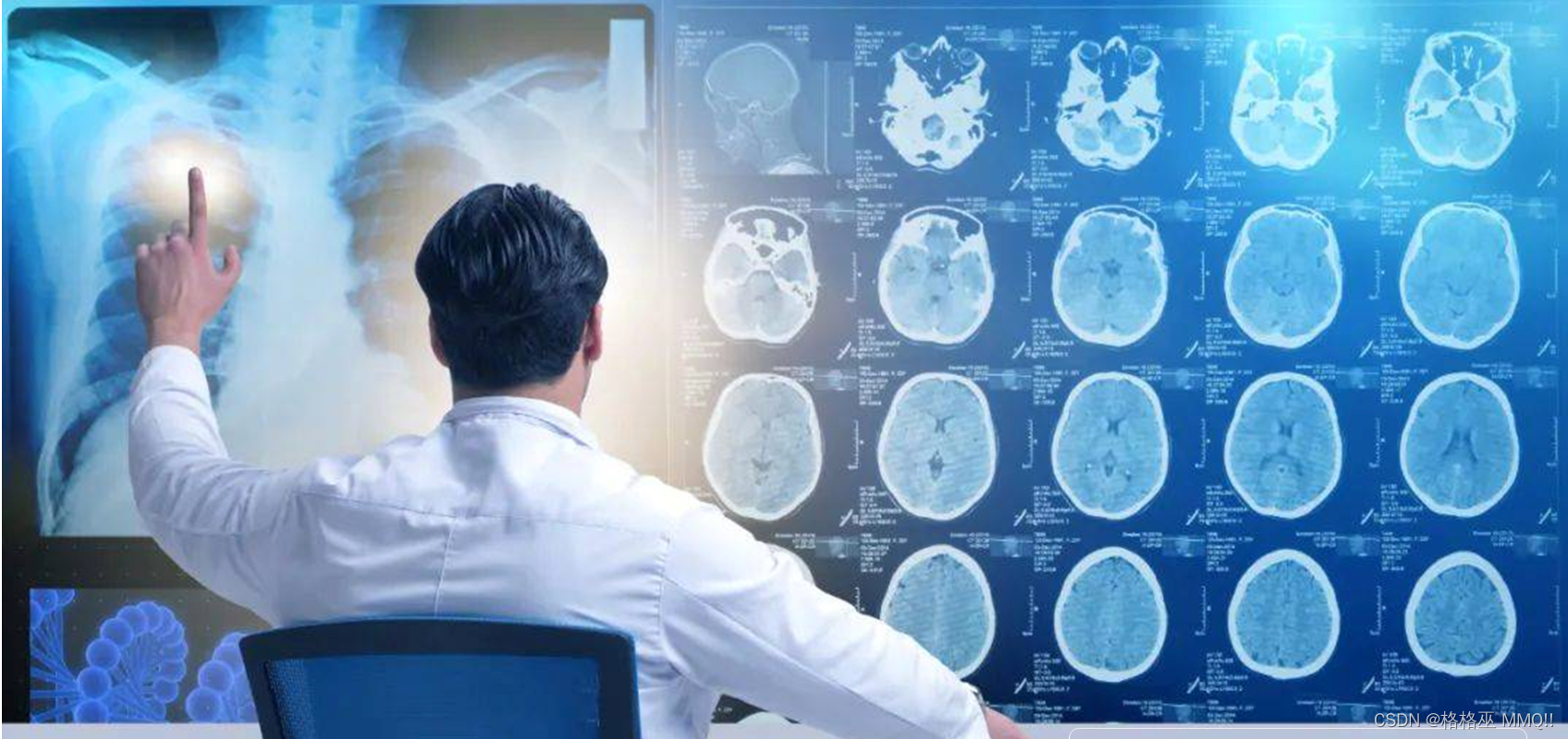
图像分割
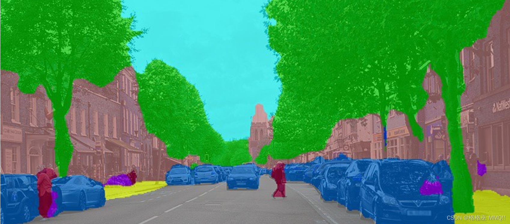
图像分割是将图像按照内容物切分为不同组的过程,它定位出了图像中的对象和边界。语义分割是像素级别的识别,我们在很多领域的典型应用,背后的技术支撑都是图像分割算法,比如:医学影像、无人驾驶可行驶区域检测、背景虚化等。
语义分割典型网络 U-Net
U-Net 是一种卷积网络架构,用于快速、精确地分割生物医学图像。
关于语义分割的各类算法原理及优缺点对比(包括U-Net),ShowMeAI 在过往文章 深度学习与CV教程(14) | 图像分割 (FCN,SegNet,U-Net,PSPNet,DeepLab,RefineNet) 中有详细详解。
U-Net 的结构如下图所示: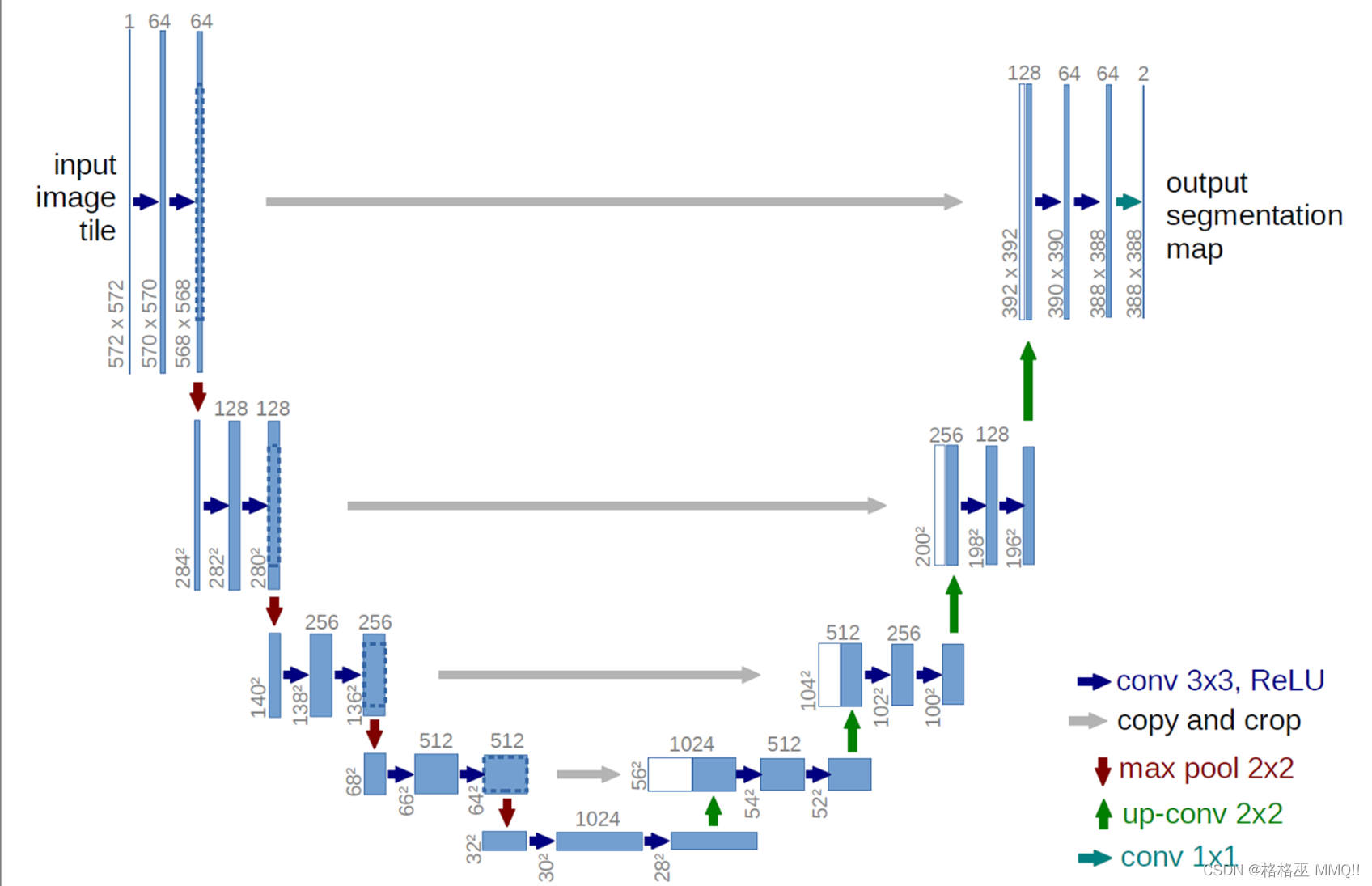
在 U-Net 中,与其他所有卷积神经网络一样,它由卷积和最大池化等层次组成。
U-Net 简单地将编码器的特征图拼接至每个阶段解码器的上采样特征图,从而形成一个梯形结构。该网络非常类似于 Ladder Network 类型的架构。
通过跳跃 拼接 连接的架构,在每个阶段都允许解码器学习在编码器池化中丢失的相关特征。
上采样采用转置卷积。
使用 U-Net 进行肺部影像分割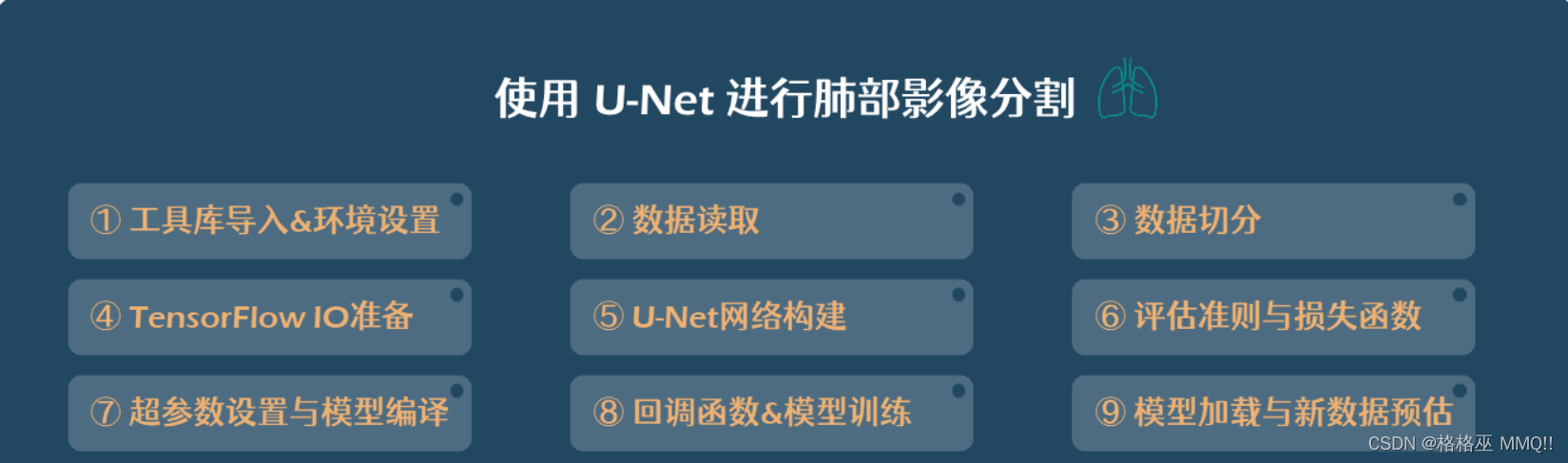
我们这里使用到的数据集是 蒙哥马利县 X 射线医学数据集。 该数据集由肺部的各种 X 射线图像以及每个 X 射线的左肺和右肺的分段图像的图像组成。大家也可以直接通过ShowMeAI的百度网盘链接下载此数据集。
工具库导入&环境设置
首先导入我们本次使用到的工具库。
导入工具库
import os
import numpy as np
import cv2
from glob import glob
from sklearn.model_selection import train_test_split
import tensorflow as tf
from tensorflow.keras.callbacks import ModelCheckpoint, ReduceLROnPlateau
from tensorflow.keras.optimizers import Adam
from tensorflow.keras.metrics import Recall, Precision
② 数据读取
接下来我们完成数据读取部分,这里读取的内容包括图像和蒙版(mask,即和图片同样大小的标签)。我们会调整维度大小,以便可以作为 U-Net 的输入。
读取X射线图像
def imageread(path,width=512,height=512):
x = cv2.imread(path, cv2.IMREAD_COLOR)
x = cv2.resize(x, (width, height))
x = x/255.0
x = x.astype(np.float32)
return x
读取标签蒙版
def maskread(path_l, path_r,width=512,height=512):
x_l = cv2.imread(path_l, cv2.IMREAD_GRAYSCALE)
x_r = cv2.imread(path_r, cv2.IMREAD_GRAYSCALE)
x = x_l + x_r
x = cv2.resize(x, (width, height))
x = x/np.max(x)
x = x > 0.5
x = x.astype(np.float32)
x = np.expand_dims(x, axis=-1)
return x
③ 数据切分
我们要对模型的效果进行有效评估,所以接下来我们进行数据划分,我们把全部数据分为训练集、验证集和测试集。具体代码如下:
“”“加载与切分数据”“”
def load_data(path, split=0.1):
images = sorted(glob(os.path.join(path, “CXR_png”, “.png")))
masks_l = sorted(glob(os.path.join(path, “ManualMask”, “leftMask”, ".png”)))
masks_r = sorted(glob(os.path.join(path, “ManualMask”, “rightMask”, “*.png”)))
split_size = int(len(images) * split) # 9:1的比例切分
train_x, val_x = train_test_split(images, test_size=split_size, random_state=42)
train_y_l, val_y_l = train_test_split(masks_l, test_size=split_size, random_state=42)
train_y_r, val_y_r = train_test_split(masks_r, test_size=split_size, random_state=42)
train_x, test_x = train_test_split(train_x, test_size=split_size, random_state=42)
train_y_l, test_y_l = train_test_split(train_y_l, test_size=split_size, random_state=42)
train_y_r, test_y_r = train_test_split(train_y_r, test_size=split_size, random_state=42)
return (train_x, train_y_l, train_y_r), (val_x, val_y_l, val_y_r), (test_x, test_y_l, test_y_r)
④ TensorFlow IO准备
我们会使用到 TensorFlow 进行训练和预估,我们用 TensorFlow 读取 numpy array 格式的数据,转为 TensorFlow 的 tensor 形式,并构建方便以 batch 形态读取和训练的 dataset 格式。
tensor格式转换
def tf_parse(x, y_l, y_r):
def _parse(x, y_l, y_r):
x = x.decode()
y_l = y_l.decode()
y_r = y_r.decode()
x = imageread(x)
y = maskread(y_l, y_r)
return x, y
x, y = tf.numpy_function(_parse, [x, y_l, y_r], [tf.float32, tf.float32])
x.set_shape([512, 512, 3])
y.set_shape([512, 512, 1])
return x, y
构建tensorflow dataset
def tf_dataset(X, Y_l, Y_r, batch=8):
dataset = tf.data.Dataset.from_tensor_slices((X, Y_l, Y_r))
dataset = dataset.shuffle(buffer_size=200)
dataset = dataset.map(tf_parse)
dataset = dataset.batch(batch)
dataset = dataset.prefetch(4)
return dataset
⑤ U-Net 网络构建
下面我们构建 U-Net 网络。
from tensorflow.keras.layers import Conv2D, BatchNormalization, Activation, MaxPool2D, Conv2DTranspose, Concatenate, Input
from tensorflow.keras.models import Model
一个卷积块结构
def conv_block(input, num_filters):
x = Conv2D(num_filters, 3, padding=“same”)(input)
x = BatchNormalization()(x)
x = Activation(“relu”)(x)
x = Conv2D(num_filters, 3, padding="same")(x)
x = BatchNormalization()(x)
x = Activation("relu")(x)

return x
编码器模块
def encoder_block(input, num_filters):
x = conv_block(input, num_filters)
p = MaxPool2D((2, 2))(x)
return x, p
解码器模块
def decoder_block(input, skip_features, num_filters):
x = Conv2DTranspose(num_filters, (2, 2), strides=2, padding=“same”)(input)
x = Concatenate()([x, skip_features])
x = conv_block(x, num_filters)
return x
完整的U-Net
def build_unet(input_shape):
inputs = Input(input_shape)
# 编码器部分
s1, p1 = encoder_block(inputs, 64)
s2, p2 = encoder_block(p1, 128)
s3, p3 = encoder_block(p2, 256)
s4, p4 = encoder_block(p3, 512)

b1 = conv_block(p4, 1024)

# 解码器部分
d1 = decoder_block(b1, s4, 512)
d2 = decoder_block(d1, s3, 256)
d3 = decoder_block(d2, s2, 128)
d4 = decoder_block(d3, s1, 64)

# 输出
outputs = Conv2D(1, 1, padding="same", activation="sigmoid")(d4)

model = Model(inputs, outputs, name="U-Net")
return model
⑥ 评估准则与损失函数
我们针对语义分割场景,编写评估准则 IoU 的计算方式,并构建 Dice Loss 损失函数以便在医疗场景语义分割下更针对性地训练学习。
关于IoU、mIoU等评估准则可以查看ShowMeAI的文章 深度学习与CV教程(14) | 图像分割 (FCN,SegNet,U-Net,PSPNet,DeepLab,RefineNet) 做更多了解。
关于Dice Loss损失函数的解释如下:
Dice 系数
根据 Lee Raymond Dice 命名,是一种集合相似度度量函数,通常用于计算两个样本的相似度(值范围为 [0,1]):
s=2|X∩Y||X|+|Y|
|X∩Y|表示 X 和 Y 之间的交集;|X| 和 |Y| 分别表示 X 和 Y 的元素个数。其中,分子中的系数 2,是因为分母存在重复计算 X 和 Y 之间的共同元素的原因。
针对,语义分割问题而言,X 为分割图像标准答案 GT,Y 为分割图像预测标签 Pred。
Dice 系数差异函数(Dice loss)
s=1−2|X∩Y||X|+|Y|
评估准则与损失函数的代码实现如下:
IoU计算
def iou(y_true, y_pred):
def f(y_true, y_pred):
intersection = (y_true * y_pred).sum()
union = y_true.sum() + y_pred.sum() - intersection
x = (intersection + 1e-15) / (union + 1e-15)
x = x.astype(np.float32)
return x
return tf.numpy_function(f, [y_true, y_pred], tf.float32)
Dice Loss定义
smooth = 1e-15
def dice_coef(y_true, y_pred):
y_true = tf.keras.layers.Flatten()(y_true)
y_pred = tf.keras.layers.Flatten()(y_pred)
intersection = tf.reduce_sum(y_true * y_pred)
return (2. * intersection + smooth) / (tf.reduce_sum(y_true) + tf.reduce_sum(y_pred) + smooth)
def dice_loss(y_true, y_pred):
return 1.0 - dice_coef(y_true, y_pred)
⑦ 超参数设置与模型编译
接下来在开始模型训练之前,我们先敲定一些超参数,如下:
批次大型 batch size = 2
学习率 learning rate= 1e-5
迭代轮次 epoch = 30
我们使用 Adam 优化器进行训练,使用的评估指标包括 Dice 系数、IoU、召回率和精度。
超参数
batch_size = 2
lr = 1e-5
epochs = 30
model_path = “models/model.h5”
读取数据
dataset_path = ‘./NLM-MontgomeryCXRSet/MontgomerySet’
(train_x, train_y_l, train_y_r), (val_x, val_y_l, val_y_r), (test_x, test_y_l, test_y_r) = load_data(dataset_path)
训练集与验证集
train_dataset = tf_dataset(train_x, train_y_l, train_y_r, batch=batch_size)
val_dataset = tf_dataset(val_x, val_y_l, val_y_r, batch=batch_size)
构建模型
model = build_unet((512, 512, 3))
评估准则
metrics = [dice_coef, iou, Recall(), Precision()]
编译模型
model.compile(loss=dice_loss, optimizer=Adam(lr), metrics=metrics)
可以使用model.summary查看模型结构信息与参数量:
model . summary()
结果如下图所示(部分内容截图,全部模型信息较长):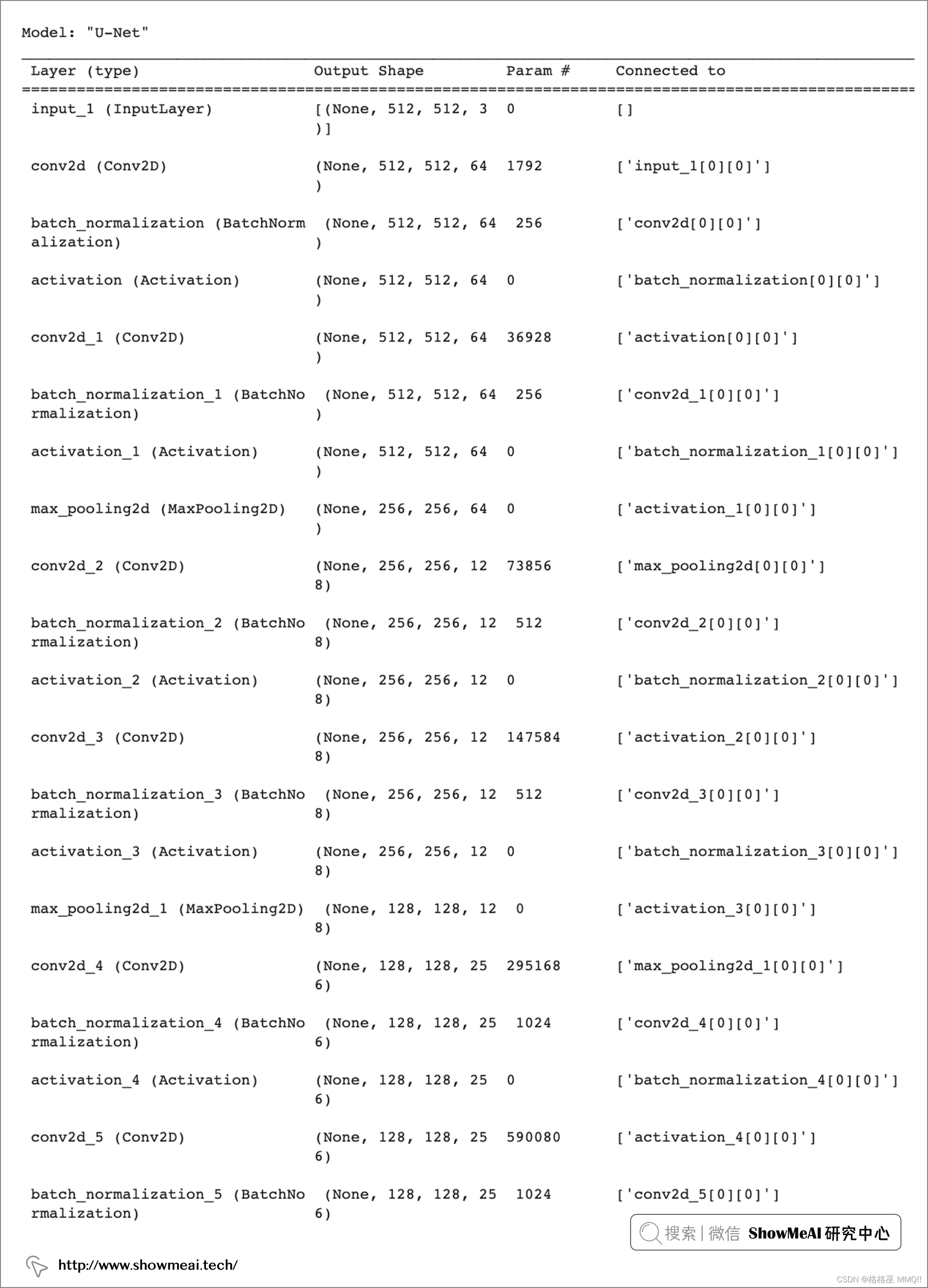
⑧ 回调函数&模型训练
我们在回调函数中设置模型存储相关设置,学习率调整策略等,之后在数据集上进行训练。
回调函数
callbacks = [
ModelCheckpoint(model_path, verbose=1, save_best_only=True),
ReduceLROnPlateau(monitor=‘val_loss’, factor=0.1, patience=5, min_lr=1e-8, verbose=1)
]
模型训练
history = model.fit(
train_dataset,
epochs=epochs,
validation_data=val_dataset,
callbacks=callbacks
)
训练部分中间信息如下图所示。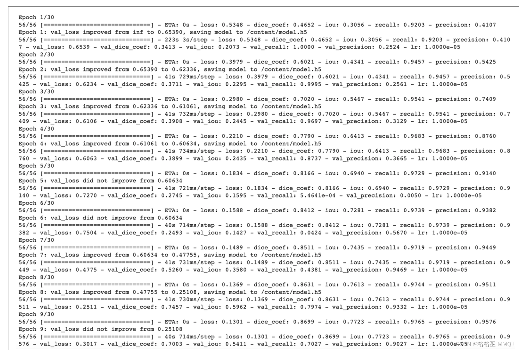
在训练模型超过 30 个 epoch 后,保存的模型(验证损失为 0.10216)相关的评估指标结果如下:
dice coef:0.9148
iou:0.8441
recall:0.9865
precision:0.9781
val_loss:0.1022
val_dice_coef: 0.9002
val_iou:0.8198
val_recall:0.9629
val_precision:0.9577
⑨ 模型加载与新数据预估
我们可以把刚才保存好的模型重新加载入内存,并对没有见过的测试数据集进行预估,代码如下:
重新载入模型
from tensorflow.keras.utils import CustomObjectScope
with CustomObjectScope({‘iou’: iou, ‘dice_coef’: dice_coef, ‘dice_loss’: dice_loss}):
model = tf.keras.models.load_model(“/content/model.h5”)
测试集预估
from tqdm import tqdm
import matplotlib.pyplot as plt
ct=0
遍历测试集
for x, y_l, y_r in tqdm(zip(test_x, test_y_l, test_y_r), total=len(test_x)):
“”" Extracing the image name. “”"
image_name = x.split(“/”)[-1]
# 读取测试图片集
ori_x = cv2.imread(x, cv2.IMREAD_COLOR)
ori_x = cv2.resize(ori_x, (512, 512))
x = ori_x/255.0
x = x.astype(np.float32)
x = np.expand_dims(x, axis=0)

# 读取标签信息
ori_y_l = cv2.imread(y_l, cv2.IMREAD_GRAYSCALE)
ori_y_r = cv2.imread(y_r, cv2.IMREAD_GRAYSCALE)
ori_y = ori_y_l + ori_y_r
ori_y = cv2.resize(ori_y, (512, 512))
ori_y = np.expand_dims(ori_y, axis=-1)  # (512, 512, 1)
ori_y = np.concatenate([ori_y, ori_y, ori_y], axis=-1)  # (512, 512, 3)

# 预估
y_pred = model.predict(x)[0] > 0.5
y_pred = y_pred.astype(np.int32)
#plt.imshow(y_pred)

# 存储预估结果mask
save_image_path = "./"+str(ct)+".png"
ct+=1
y_pred = np.concatenate([y_pred, y_pred, y_pred], axis=-1)
sep_line = np.ones((512, 10, 3)) * 255
cat_image = np.concatenate([ori_x, sep_line, ori_y, sep_line, y_pred*255], axis=1)
cv2.imwrite(save_image_path, cat_image)
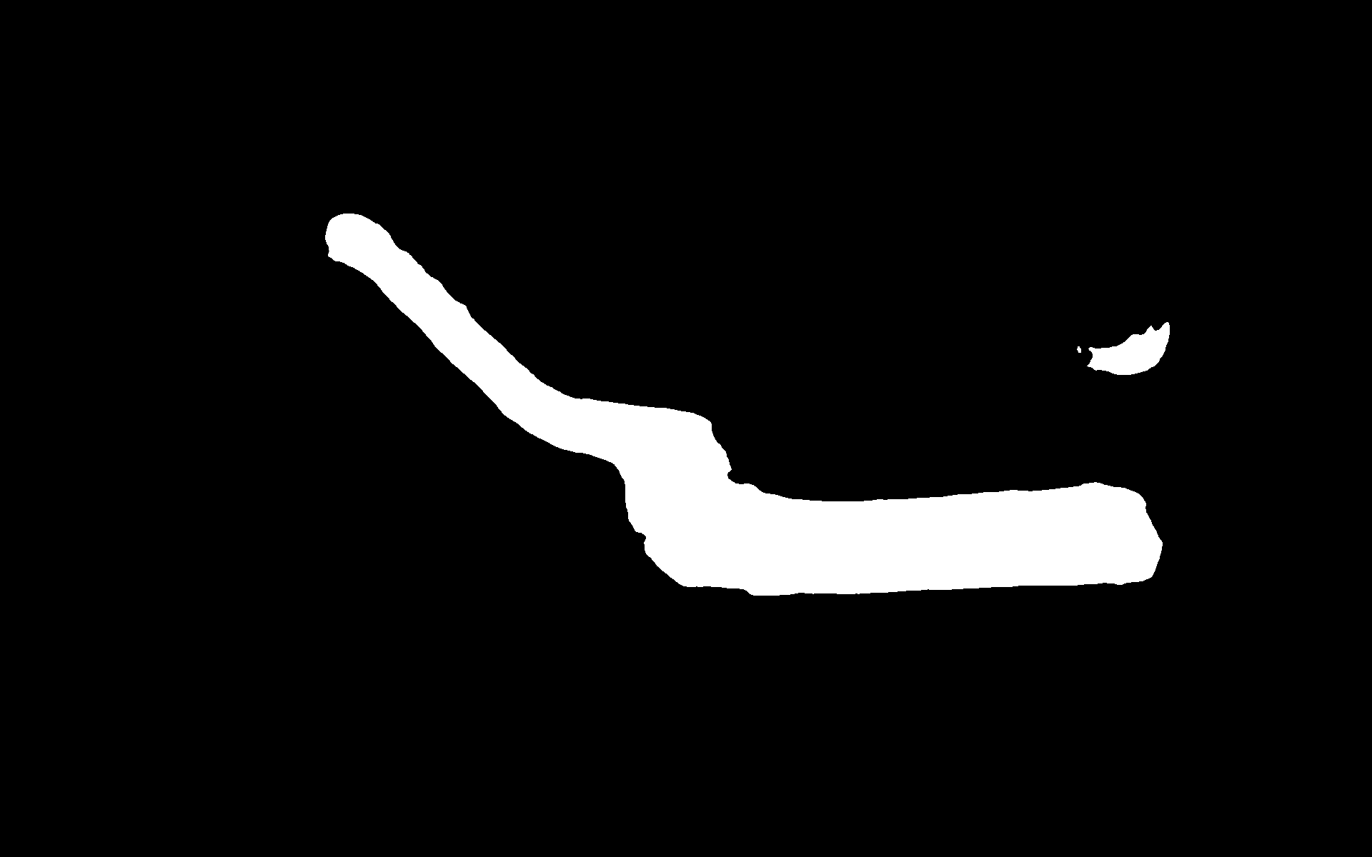
部分结果可视化:
下面为2个测试样本的原始图像、原始掩码(标准答案)和预测掩码的组合图像:
测试用例的输入图像(左侧)、原始掩码标签(中间)、预测掩码(右侧)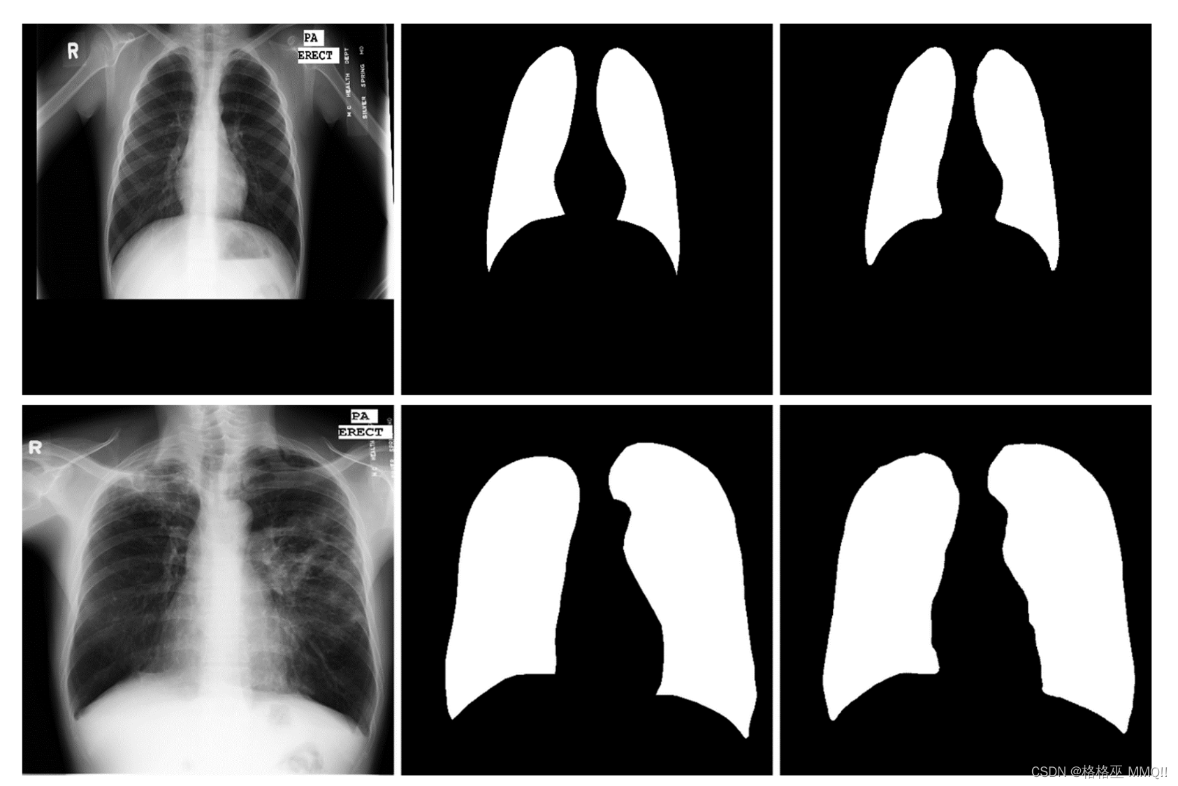
边栏推荐
猜你喜欢
随机推荐
CCF大会腾源会专场即将召开,聚焦基础软件与开发语言未来发展
二、第二章变量
日志使用注意事项和建议
【学习笔记】线性规划对偶定理
C# Call AutoNavi Map API to obtain latitude, longitude and positioning [Detailed 4D explanation with complete code]
【2022】【Thesis Notes】Ultra-thin THz deflection based on laser direct writing graphene oxide paper——
齐话存储未来,诠释分布式缘起
开发者时薪高达1200美元?一文带你走近Move语言的编程魅力!
悠漓带你玩转C语言(详解操作符1)
突破次元壁垒,让身边的玩偶手办在屏幕上动起来!
【学习笔记】一般图最大匹配
SDUT数据库 SQL语句练习(MySQL)
宝塔计划任务执行周期设置【秒】为定时单位【或者更小】
LeetCode每日一题(1754. Largest Merge Of Two Strings)
5. 内部类
1.TCP/IP基础知识
form-making notes on climbing pits (jeecg project replaces form designer)
【综合练习12】实现静态网页的相关功能
从零开始配置 vim(12)——主题配置
openEuler小程序会议指南