当前位置:网站首页>[numerical prediction case] (3) LSTM time series electricity quantity prediction, with tensorflow complete code attached
[numerical prediction case] (3) LSTM time series electricity quantity prediction, with tensorflow complete code attached
2022-04-23 19:46:00 【Vertical sir】
Hello everyone , Today I'd like to share with you how to use recurrent neural network LSTM Complete time series prediction , This paper is a prediction for a single feature , The next article is the prediction of multiple features . There is a complete code at the end of the text
1. Import toolkit
Use here GPU Accelerate Computing , Speed up network training .
import tensorflow as tf
from tensorflow import keras
import numpy as np
import pandas as pd
import matplotlib.pyplot as plt
import warnings
warnings.filterwarnings('ignore')
#  call GPU Speed up
gpus = tf.config.experimental.list_physical_devices(device_type='GPU')
for gpu in gpus:
    tf.config.experimental.set_memory_growth(gpu, True)
2. Get data set
The data set needs to be self fetched :https://pan.baidu.com/s/1uWW7w1Ci04U3d8YFYPf3Cw Extraction code :00qw
With the help of pandas The library reads the electric quantity time series data , Two columns of characteristic data , Time and power
#(1) get data , At intervals 1h Recorded power data
filepath = 'energy.csv'
data = pd.read_csv(filepath)
print(data.head())

3. Data preprocessing
Because it is a prediction based on time series , Change the index in the data into time , take AFP The electric quantity characteristic column is used as the characteristic of training .
Due to the large difference between the maximum and minimum of the original data , In order to avoid data affecting the stability of network training , Standardize the characteristic data for training .
#(3) Select features
temp = data['AEP_MW'] #  Get power data
temp.index = data['Datetime'] #  Change the index to time series
temp.plot()  #  Graphic display

#(4) Preprocess the training set
temp_mean = temp[:train_num].mean()  #  mean value
temp_std = temp[:train_num].std()  #  Standard deviation
#  Standardization
inputs_feature = (temp - temp_mean) / temp_std
Draw the original data distribution map

4. Divide the data set
First , need Select the eigenvalue and its corresponding tag value through the sliding window of time series . For example, predict a certain point in time , Every provision 20 Eigenvalues , Predict a tag value . Because there is only one column of characteristic data , amount to , Before use 20 Data forecast No 21 Data . Similarly, predict a certain time segment , Use the first 1 To 20 Data forecast No 21 To 30 The electricity .
#(2) Build time series sampling function
'''
dataset For the input characteristic data , Choose which features to use
start_index  With so much data, choose which to start with , Generally from 0 Start fetching sequence
history_size Indicates the size of the time window ; if 20, It means to find... From the starting index 20 Take a sample as x, The next index is treated as y
target_size Indicates the time point after the window when the predicted result is needed ;0 Indicates the prediction result at the next time point , Take it as a label ; If it is a sequence , An indicator that predicts a sequence
indices=range(i, i+history_size)  Represents the index of the window sequence ,i The starting position of each window is indicated , Index of all data in the window
'''
def database(dataset, start_index, end_index, history_size, target_size):
    data = []  #  Store eigenvalues
    labels = []  #  Store the target value

    #  Initial value segment [0:history_size]
    start_index = start_index + history_size

    #  If the eigenvalue is not specified, terminate the index , Just before the last partition
    if end_index is None:
        end_index = len(dataset) - target_size

    #  Traverse the entire power data , Extract the feature and its corresponding prediction target
    for i in range(start_index, end_index):
        indices = range(i - history_size, i) #  Index of all elements in the window
        #  Save characteristic values and label values
        data.append(np.reshape(dataset[indices], (history_size, 1)))
        labels.append(dataset[i+target_size]) #  Predict the weather data of several segments in the future
    #  Return data set
    return np.array(data), np.array(labels)
Next, you can divide... In the original data set Training set 、 Verification set 、 Test set , Respective proportion 90:9.8:0.2
#  Take before 90% Data as a training set
train_num = int(len(data) * 0.90)
# 90%-99.8% Used to verify
val_num = int(len(data) * 0.998)
#  Last 1% Used for testing

#(5) Divide training set and verification set
#  The window is 20 Data , Predict the temperature at the next moment
history_size = 20
target_size=0

#  Training set
x_train, y_train = database(inputs_feature.values, 0, train_num,
                            history_size, target_size)

#  Verification set
x_val, y_val = database(inputs_feature.values, train_num, val_num,
                          history_size, target_size)

#  Test set
x_test, y_test = database(inputs_feature.values, val_num, None,
                          history_size, target_size)

#  View data information
print('x_train.shape:', x_train.shape)  # x_train.shape: (109125, 20, 1)
5. Construct data set
Will divide the good numpy The training set and verification set of type are converted to tensor type , For network training . Use shuffle() Function scrambles the training set data ,batch() The function specifies each step How many sets of data to train . With the help of iterator iter() Use next() Functions from the dataset Take out a batch The data of Used to verify .
#(6) structure tf Data sets
#  Training set
train_ds = tf.data.Dataset.from_tensor_slices((x_train, y_train))
train_ds = train_ds.shuffle(10000).batch(128)
#  Verification set
val_ds = tf.data.Dataset.from_tensor_slices((x_val, y_val))
val_ds = val_ds.batch(128)

#  View data information
sample = next(iter(train_ds))
print('x_batch.shape:', sample[0].shape, 'y_batch.shape:', sample[1].shape)
print('input_shape:', sample[0].shape[-2:])
# x_batch.shape: (128, 20, 1) y_batch.shape: (128,)
# input_shape: (20, 1)
6. model building
Due to the small amount of data in this case , There is only one feature , Therefore, there is no need to use complex networks , Use one LSTM Layers are used to extract features , A full connection layer is used to output the prediction results .
#  Construct input layer
inputs = keras.Input(shape=sample[0].shape[-2:])
#  Build all layers of the network
x = keras.layers.LSTM(8)(inputs)
x = keras.layers.Activation('relu')(x)
outputs = keras.layers.Dense(1)(x)  #  The output is 1 individual
#  Build a model
model = keras.Model(inputs, outputs)
#  Look at the model structure
model.summary()
The network architecture is as follows :
Layer (type)                 Output Shape              Param #
=================================================================
input_1 (InputLayer)         [(None, 20, 1)]           0
_________________________________________________________________
lstm_1 (LSTM)                (None, 8)                 320
_________________________________________________________________
activation_1 (Activation)    (None, 8)                 0
_________________________________________________________________
dense_1 (Dense)              (None, 1)                 9
=================================================================
Total params: 329
Trainable params: 329
Non-trainable params: 0
7. Network training
First, compile the model , Use adam The optimizer sets the learning rate 0.01, The average absolute error is used as the loss function of network training , Network iteration 20 Time . Regression problem cannot be set metrics The monitoring index is accuracy , This is generally used for classification problems .
#(8) Model compilation
opt = keras.optimizers.Adam(learning_rate=0.001)  #  Optimizer

model.compile(optimizer=opt, loss='mae')  #  Average error loss

#(9) model training
epochs=20
history = model.fit(train_ds, epochs=epochs, validation_data=val_ds)
The training process is as follows :
Epoch 1/20
853/853 [==============================] - 5s 5ms/step - loss: 0.4137 - val_loss: 0.0878
Epoch 2/20
853/853 [==============================] - 4s 5ms/step - loss: 0.0987 - val_loss: 0.0754
---------------------------------------------------
---------------------------------------------------
Epoch 19/20
853/853 [==============================] - 4s 5ms/step - loss: 0.0740 - val_loss: 0.0607
Epoch 20/20
853/853 [==============================] - 4s 4ms/step - loss: 0.0736 - val_loss: 0.0628
8. View workout info
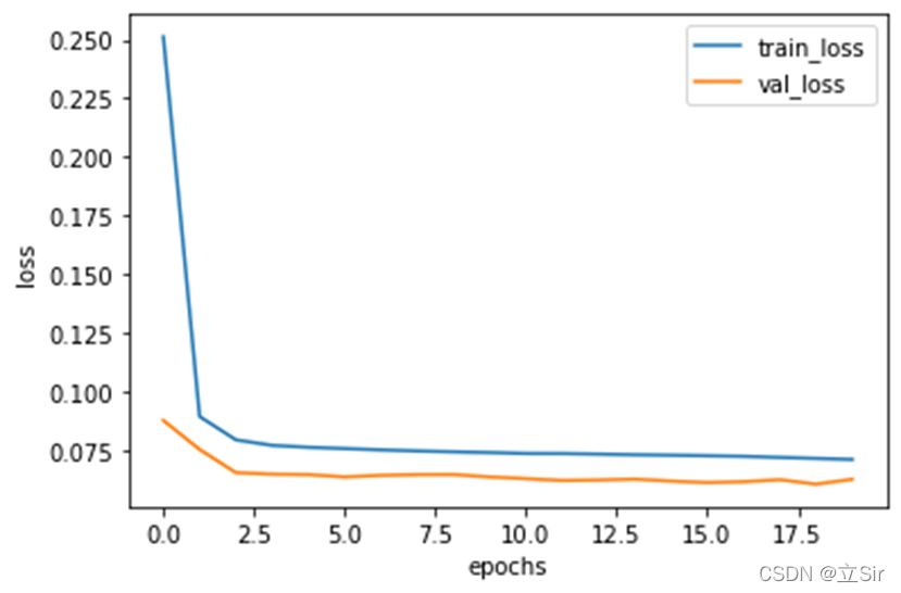
history All the information of the training process is saved in the variable , We draw the loss curve of training set and verification set .
#(10) Get training information
history_dict = history.history  #  Get the training data dictionary
train_loss = history_dict['loss']  #  Training set loss
val_loss = history_dict['val_loss']  #  Verification set loss

#(11) Draw training loss and verification loss
plt.figure()
plt.plot(range(epochs), train_loss, label='train_loss')  #  Training set loss
plt.plot(range(epochs), val_loss, label='val_loss')  #  Verification set loss
plt.legend()  #  Show labels
plt.xlabel('epochs')
plt.ylabel('loss')
plt.show()
9. Prediction stage
Predict the previously divided test set ,model The weight of network training is saved in , Use predict() function Predictive features x_test The corresponding electric quantity y_predict, True value y_test, The plot shows the degree of deviation between the predicted value and the real value . You can also calculate the variance or standard deviation between the predicted value and the real value to show the accuracy of the prediction .
#(12) forecast
y_predict = model.predict(x_test)  #  Predict the eigenvalues of the test set

# x_test  Equivalent to pretreated  temp[val_num:-20].values
dates = temp[val_num:-20].index  #  Get time index

#(13) Draw a comparison diagram between the predicted results and the real values
fig = plt.figure(figsize=(10,5))
#  True value
axes = fig.add_subplot(111)
axes.plot(dates, y_test, 'bo', label='actual')
#  Predictive value , Red scatter
axes.plot(dates, y_predict, 'ro', label='predict')
#  Set the abscissa scale
axes.set_xticks(dates[::30])
axes.set_xticklabels(dates[::30],rotation=45)

plt.legend()  #  notes
plt.grid()  #  grid
plt.show()
because x_test The corresponding index in the original data is val_num Later feature information , find x_test The time corresponding to each element in the dates, As x Axis scale

版权声明
本文为[Vertical sir]所创,转载请带上原文链接,感谢
https://yzsam.com/2022/04/202204231930160458.html
边栏推荐
- Easy mock local deployment (you need to experience three times in a crowded time. Li Zao will do the same as me. Love is like a festival mock)
- ESP8266-入门第一篇
- Codeworks round 783 (Div. 2) d problem solution
- Speex Wiener filter and rewriting of hypergeometric distribution
- Design of warehouse management database system
- Data analysis learning directory
- Electron入门教程3 ——进程通信
- Project training of Software College of Shandong University - Innovation Training - network security shooting range experimental platform (VII)
- [transfer] summary of new features of js-es6 (one picture)
- The usage of slice and the difference between slice and array
猜你喜欢

An algorithm problem was encountered during the interview_ Find the mirrored word pairs in the dictionary
2021-2022-2 ACM training team weekly Programming Competition (8) problem solution
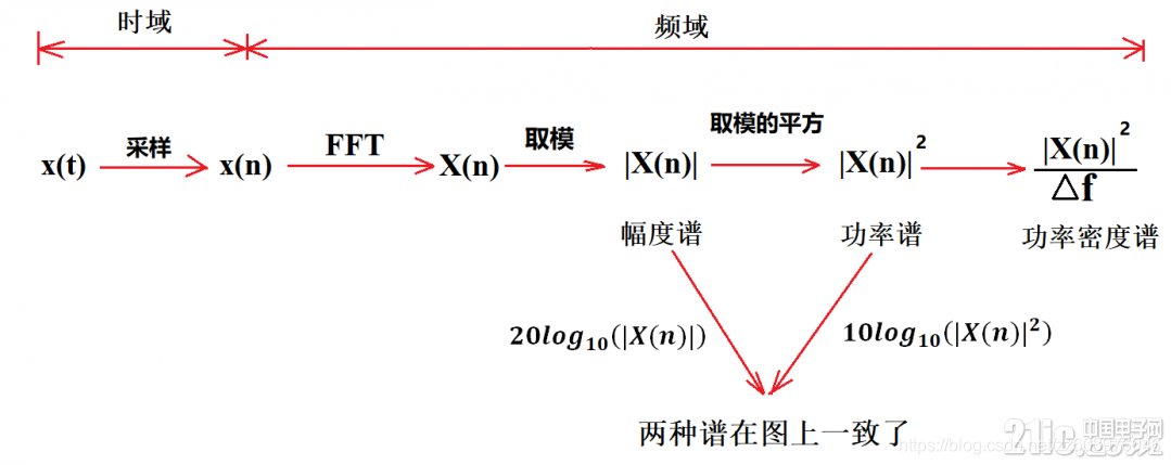
Physical meaning of FFT: 1024 point FFT is 1024 real numbers. The actual input to FFT is 1024 complex numbers (imaginary part is 0), and the output is also 1024 complex numbers. The effective data is
如何在BNB链上创建BEP-20通证
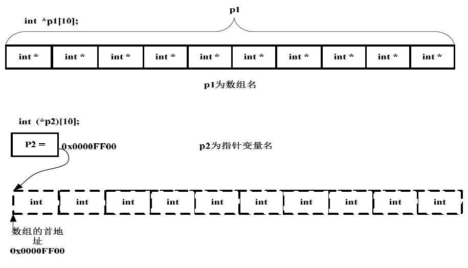
指针数组与数组指针的区分
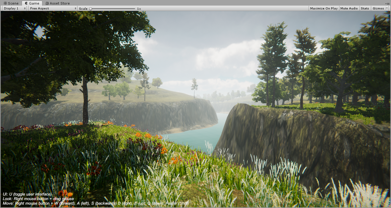
Unity创建超写实三维场景的一般步骤
Unity general steps for creating a hyper realistic 3D scene
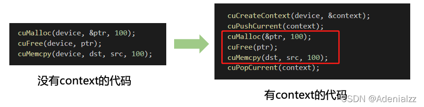
精简CUDA教程——CUDA Driver API

Understanding various team patterns in scrum patterns
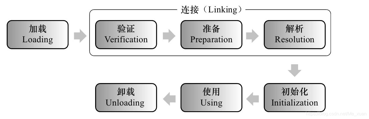
Class loading mechanism
随机推荐
php参考手册String(7.2千字)
MySQL数据库 - 数据库和表的基本操作(二)
【数值预测案例】(3) LSTM 时间序列电量预测,附Tensorflow完整代码
Shanda Wangan shooting range experimental platform project - personal record (V)
MySQL syntax collation (5) -- functions, stored procedures and triggers
Core concepts of rest
Speex维纳滤波与超几何分布的改写
The usage of slice and the difference between slice and array
Mysql database - single table query (II)
Possible root causes include a too low setting for -Xss and illegal cyclic inheritance dependencies
JVM的类加载过程
Pdf reference learning notes
基于pytorch搭建GoogleNet神经网络用于花类识别
MFCC: Mel频率倒谱系数计算感知频率和实际频率转换
【webrtc】Add x264 encoder for CEF/Chromium
uIP1.0 主动发送的问题理解
什么是消息队列
Devops integration - environment variables and building tools of Jenkins service
TI DSP的 FFT与IFFT库函数的使用测试
【h264】libvlc 老版本的 hevc h264 解析,帧率设定