【机器学习】数据科学基础——Machine Learning Fundamentals Practice（二）

活动地址：[CSDN21天学习挑战赛](https://marketing.csdn.net/p/bdabfb52c5d56532133df2adc1a728fd)

作者简介：在校大学生一枚,华为云享专家,阿里云星级博主,腾云先锋（TDP）成员,The general manager of Yunxi Smart Project,National Committee of Experts on Computer Teaching and Industrial Practice Resource Construction in Colleges and Universities（TIPCC）志愿者,and programming enthusiasts,期待和大家一起学习,一起进步~
.
博客主页：ぃ灵彧が的学习日志
.
本文专栏：机器学习
.
专栏寄语：若你决定灿烂,山无遮,海无拦
.

前言

什么是机器学习？

Machine learning is an important branch in the field of artificial intelligence,intended by means of computation,Use experience to improve the performance of computer systems,通常,The experience here is historical data.Abstract an algorithm model from a large amount of data,Then feed the data into the model,Get the model's judgment on it（例如类型、Predict real values, etc）,也就是说,Machine learning is a discipline that mainly studies learning algorithms.

一、Text classification based on Naive Bayes

导读：

贝叶斯分类算法It is a series of classification algorithms based on Bayes' theorem,Contains Naive Bayes and Tree Augmented Bayes,Naive Bayes is the simplest yet very efficient Bayesian classification algorithm,Because it assumes that the input features are independent of each other,因此得名“朴素”.

模型选择：

贝叶斯分类： 贝叶斯分类是一类分类算法的总称,这类算法均以贝叶斯定理为基础,故统称为贝叶斯分类.

贝叶斯公式: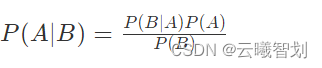

​
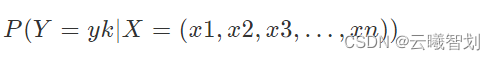
在**文本分类（classification）**问题中,We want to classify a sentence into a certain category,We consider the words or characters in a sentence as properties of the sentence,So a sentence is composed of attributes（字/词）组成的,Think of many attributes as a vector,即X=(x1,x2,x3,…,xn),用XThis vector to represent the sentence. 类别也有很多种,我们用集合Y={y1,y2,…ym}表示.

A sentence belongs toykThe probability of a class can be expressed as ：

If the attribute vector of a sentenceX属于ykThe class has the highest probability,即：

其中,X=(x1,x2,x3,…,xn),可以给X打上yk标签,意思是说X属于yk类别.This is called classification(Classification).

朴素贝叶斯：

假设X=(x1,x2,x3,…,xn)All properties in are independent,即

The introduction of Laplace smoothing：

If the conditional probability of an attribute is 0,would result in an overall probability of zero,为了避免这种情况出现,Introduce the Laplace smoothing parameter,That is, the conditional probability is 0The probability of the attribute is set to a fixed value.

(一)、数据加载及预处理

1. 导入相关包：

#导入必要的包
import random
import jieba  # 处理中文
from sklearn import model_selection
from sklearn.naive_bayes import MultinomialNB
import re,string

2. 加载文本,Filter special characters in it

def text_to_words(file_path):
    ''' 分词 return:sentences_arr, lab_arr '''
    sentences_arr = []
    lab_arr = []
    with open(file_path,'r',encoding='utf8') as f:
        for line in f.readlines():
            lab_arr.append(line.split('_!_')[1])
            sentence = line.split('_!_')[-1].strip()
            sentence = re.sub("[\s+\.\!\/_,$%^*(+\"\')]+|[+——()?【】“”！,.？、[email protected]#￥%……&*（）《》：]+", "",sentence) #去除标点符号
            sentence = jieba.lcut(sentence, cut_all=False)
            sentences_arr.append(sentence)
    return sentences_arr, lab_arr

3. 加载停用词表,Count the frequency of text words,Filter out stop words and words with low word frequency,构建词表：

def load_stopwords(file_path):
    ''' 创建停用词表 参数 file_path:停用词文本路径 return：停用词list '''
    stopwords = [line.strip() for line in open(file_path, encoding='UTF-8').readlines()]
    return stopwords

def get_dict(sentences_arr,stopswords):
    ''' 遍历数据,去除停用词,统计词频 return: 生成词典 '''
    word_dic = {
    }
    for sentence in sentences_arr:
        for word in sentence:
            if word != ' ' and word.isalpha():
                if word not in stopswords:
                    word_dic[word] = word_dic.get(word,1) + 1
    word_dic=sorted(word_dic.items(),key=lambda x:x[1],reverse=True) #Sort by word frequency

    return word_dic

4. Pick from dictionaryN个特征词,Form a list of feature words.

def get_feature_words(word_dic,word_num):
    ''' Pick from dictionaryN个特征词,Form a list of feature words return: 特征词列表 '''
    n = 0
    feature_words = []
    for word in word_dic:
        if n < word_num:
            feature_words.append(word[0])
        n += 1
    return feature_words

# 文本特征
def get_text_features(train_data_list, test_data_list, feature_words):
    ''' According to feature words,Convert the sentences in the dataset into feature vectors '''
    def text_features(text, feature_words):
        text_words = set(text)
        features = [1 if word in text_words else 0 for word in feature_words] # 形成特征向量
        return features
    train_feature_list = [text_features(text, feature_words) for text in train_data_list]
    test_feature_list = [text_features(text, feature_words) for text in test_data_list]
    return train_feature_list, test_feature_list

#Get the segmented data and labels
sentences_arr, lab_arr = text_to_words('data/data6826/news_classify_data.txt')
#加载停用词
stopwords = load_stopwords('data/data43470/stopwords_cn.txt')
# 生成词典
word_dic = get_dict(sentences_arr,stopwords)
#数据集划分
train_data_list, test_data_list, train_class_list, test_class_list = model_selection.train_test_split(sentences_arr, 
                                                                                                      lab_arr, 
                                                                                                      test_size=0.1)
#Generate a list of feature words
feature_words =  get_feature_words(word_dic,10000)

#生成特征向量
train_feature_list,test_feature_list = get_text_features(train_data_list,test_data_list,feature_words)

(二)、模型定义与训练

in the above probability calculation,There may be a word that never occurs in a certain type,That is, the conditional probability of an attribute is 0(P(x|c)=0),This results in an overall probability of zero,为了避免这种情况出现,Introduce the Laplace smoothing parameter,Set the conditional probability to be 0The probability of the attribute is set to a fixed value,具体的,Add the counts of all words under each type1,When the number of training sample sets is sufficiently large,并不会对结果产生影响.In the parameters of the following call interface,alpha为1时,Indicates that Laplace smoothing is used,若设置为0,Smoothing is not used;fit_priorRepresents whether to learn prior probabilitiesP(Y=c),如果设置为False,Then all sample type outputs have the same class prior probability;class_priorfor each type of prior probability,If no specific prior probability is given, it is automatically calculated based on the data.

代码如下：

from sklearn.metrics import accuracy_score,classification_report
#Get the Naive Bayes classifier
classifier = MultinomialNB(alpha=1.0,  # 拉普拉斯平滑
                          fit_prior=True,  #Whether to consider prior probabilities
                          class_prior=None)

#进行训练 
classifier.fit(train_feature_list, train_class_list)

(三)、模型训练

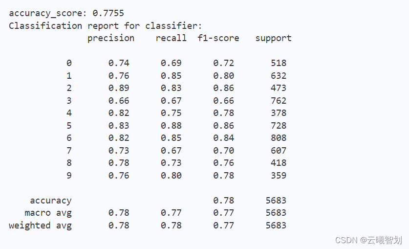
模型训练结束后,The performance of the model can be tested using the validation set,同上一小节,while outputting the accuracy,Accuracy rate for each type、召回率以及F1The value is also output.

代码如下：

# 在验证集上进行验证
predict = classifier.predict(test_feature_list)
test_accuracy = accuracy_score(predict,test_class_list)
print("accuracy_score: %.4lf"%(test_accuracy))
print("Classification report for classifier:\n",classification_report(test_class_list, predict))

输出结果如下图1-1所示：

(四)、模型预测

Use the above trained model,for any given text data,Prediction is possible,Observe the generalization performance of the model.

代码如下：

#load sentence,对句子进行预处理
def load_sentence(sentence):
    sentence = re.sub("[\s+\.\!\/_,$%^*(+\"\')]+|[+——()?【】“”！,.？、[email protected]#￥%……&*（）《》：]+", "",sentence) #去除标点符号
    sentence = jieba.lcut(sentence, cut_all=False)
    return sentence

lab = [ '文化', '娱乐', '体育', '财经','房产', '汽车', '教育', '科技', '国际', '证券']

p_data = '【China is moving forward steadily】To deal with risks and challenges, institutional advantages must be brought into play'
sentence = load_sentence(p_data)
sentence= [sentence]
print('分词结果:', sentence)
#形成特征向量
p_words = get_text_features(sentence,sentence,feature_words)
res = classifier.predict(p_words[0])
print("所属类型：",lab[int(res)])

The text prediction results are shown in the figure below1-2所示：

二、Luantail flower classification based on support vector product

导读：

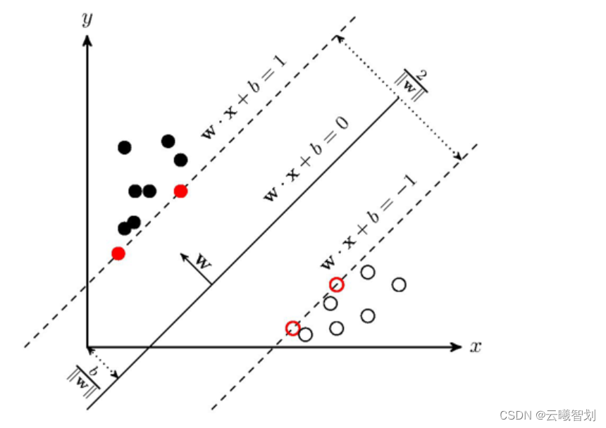
支持向量机(SVM)It is a classic classification algorithm in machine learning,The main idea is to maximize the distance sum between different types of samples to the classification hyperplane.

对于SVM,存在一个分类面,两个点集到此平面的最小距离最大,两个点集中的边缘点到此平面的距离最大.

(一)、数据加载及预处理

1. 导入相关包：

import numpy as np
from matplotlib import colors
from sklearn import svm 
from sklearn import model_selection
import matplotlib.pyplot as plt
import matplotlib as mpl

2. 加载数据、切分数据集：

# ======将字符串转化为整形==============
def iris_type(s):
    it = {
    b'Iris-setosa':0, b'Iris-versicolor':1,b'Iris-virginica':2} 
    return it[s]
    
# 1 数据准备
# 1.1 加载数据
data = np.loadtxt('/home/aistudio/data/data2301/iris.data',  # 数据文件路径i
                  dtype=float,    # 数据类型
                  delimiter=',',  # 数据分割符
                  converters={
    4:iris_type}) # 将第五列使用函数iris_type进行转换
# 1.2 数据分割
x, y = np.split(data, (4, ), axis=1) # 数据分组 第五列开始往后为y 代表纵向分割按列分割
x = x[:, :2]
x_train, x_test, y_train, y_test=model_selection.train_test_split(x, y, random_state=1, test_size=0.2)
print(x.shape,x_train.shape,x_test.shape)

(二)、模型配置

sklearn.svm.SVC()Functions provide several configurable parameters,其中,Cis the penalty coefficient for the error term.C越大,The larger the penalty for training set error terms.The higher the accuracy of the model on the training set,越容易过拟合.C越小,The more allow some misclassifications in the training samples,泛化能力强.

对于训练样本带有噪声的情况,Generally smaller ones are usedC,把训练样本集中错误分类的样本作为噪声;Kernelis the kernel function used,Default is linear kernel,An optional one-to-many classification decision function：

linear/poly/rbf/sigmoid/precomputed,decision_function_shape为ovr

# SVM分类器构建
def classifier():
    clf = svm.SVC(C=0.8,                         # 误差项惩罚系数
                  kernel='linear',               # 线性核 高斯核 rbf
                  decision_function_shape='ovr') # 决策函数
    return clf
    
# 训练模型
def train(clf, x_train, y_train):
    clf.fit(x_train, y_train.ravel()) # 训练集特征向量和 训练集目标值
   

# 2 定义模型 SVM模型定义
clf = classifier()
# 3 训练模型
train(clf, x_train, y_train)

(三)、模型训练

Test the accuracy of the model on the divided test set,The accuracy of model predictions was calculated using two methods：自定义方法show_accuracy()以及sklearnA good way to encapsulate the machine learning model in Chinasocre(),Verify the consistency of the two,and output samplesxdistance to each decision hyperplane,Select the type corresponding to the positive maximum value as the classification result.

# ======判断a,b是否相等计算acc的均值
def show_accuracy(a, b, tip):
    acc = a.ravel() == b.ravel()
    print('%s Accuracy:%.3f' %(tip, np.mean(acc)))
    
# 分别打印训练集和测试集的准确率 score(x_train, y_train)表示输出 x_train,y_train在模型上的准确率
def print_accuracy(clf, x_train, y_train, x_test, y_test):
    print('training prediction:%.3f' %(clf.score(x_train, y_train)))
    print('test data prediction:%.3f' %(clf.score(x_test, y_test)))
    # 原始结果和预测结果进行对比 predict() 表示对x_train样本进行预测,返回样本类别
    show_accuracy(clf.predict(x_train), y_train, 'traing data')
    show_accuracy(clf.predict(x_test), y_test, 'testing data')
    # 计算决策函数的值 表示x到各个分割平面的距离
    print('decision_function:\n', clf.decision_function(x_train)[:2])

(四)、模型可视化展示

To draw the spatial area corresponding to each type,A large number of sample points need to be collected,But this dataset only contains 150条数据,The area drawn is not too detailed,因此,Large-scale sample data needs to be generated,The classification area is drawn based on the generated data.

def draw(clf, x):   
    iris_feature = 'sepal length', 'sepal width', 'petal length', 'petal width'
    # 开始画图
    x1_min, x1_max = x[:, 0].min(), x[:, 0].max()
    x2_min, x2_max = x[:, 1].min(), x[:, 1].max()
    # 生成网格采样点
    x1, x2 = np.mgrid[x1_min:x1_max:200j, x2_min:x2_max:200j]  
  
    grid_test = np.stack((x1.flat, x2.flat), axis = 1)
    print('grid_test:\n', grid_test[:2])
    # 输出样本到决策面的距离
    z = clf.decision_function(grid_test)
    print('the distance to decision plane:\n', z[:2])
    grid_hat = clf.predict(grid_test)
    # 预测分类值 得到[0, 0, ..., 2, 2]
    print('grid_hat:\n', grid_hat[:2])
    # 使得grid_hat 和 x1 形状一致
    grid_hat = grid_hat.reshape(x1.shape)
    cm_light = mpl.colors.ListedColormap(['#A0FFA0', '#FFA0A0', '#A0A0FF'])
    cm_dark = mpl.colors.ListedColormap(['g', 'b', 'r'])
    plt.pcolormesh(x1, x2, grid_hat, cmap = cm_light) # 能够直观表现出分类边界

    plt.scatter(x[:, 0], x[:, 1], c=np.squeeze(y), edgecolor='k', s=50, cmap=cm_dark )
    plt.scatter(x_test[:, 0], x_test[:, 1], s=120, facecolor='none',zorder=10)
    plt.xlabel(iris_feature[0], fontsize=20) # 注意单词的拼写label
    plt.ylabel(iris_feature[1], fontsize=20)
    plt.xlim(x1_min, x1_max)
    plt.ylim(x2_min, x2_max)
    plt.title('Iris data classification via SVM', fontsize=30)
    plt.grid()
    plt.show()

# 4 模型评估
print('-------- eval ----------')
print_accuracy(clf, x_train, y_train, x_test, y_test)
# 5 模型使用
print('-------- show ----------')
draw(clf, x) 

三、基于K-meansImplement luantail flower clustering

导读：

K-meansIt is a classic unsupervised clustering algorithm,对于给定的样本集,按照样本之间的距离大小,将样本集划分为K个簇,让簇内的点尽量紧密地连在一起,而让簇间的距离尽量大.

(一)、数据加载及预处理

1. 导入相关包

import matplotlib.pyplot as plt
import numpy as np
from sklearn.cluster import KMeans 
from sklearn import datasets 

2. 直接从sklearn.datasets中加载数据集

# 直接从sklearn中获取数据集
iris = datasets.load_iris()
X = iris.data[:, :4]    # 表示我们取特征空间中的4个维度
print(X.shape)

3. 绘制二维数据分布图

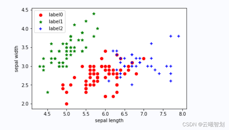
# 取前两个维度（萼片长度、萼片宽度）,绘制数据分布图
plt.scatter(X[:, 0], X[:, 1], c="red", marker='o', label='see')
plt.xlabel('sepal length')
plt.ylabel('sepal width')
plt.legend(loc=2)
plt.show() 

(二)、模型配置

实例化K-means类,And define the training function

def Model(n_clusters):
    estimator = KMeans(n_clusters=n_clusters)# 构造聚类器
    return estimator

def train(estimator):
    estimator.fit(X)  # 聚类

(三)、模型训练

训练

# 初始化实例,并开启训练拟合
estimator=Model(3)     
train(estimator)     

(四)、模型可视化展示

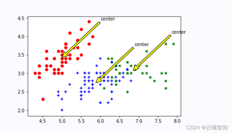
label_pred = estimator.labels_  # 获取聚类标签
# 绘制k-means结果
x0 = X[label_pred == 0]
x1 = X[label_pred == 1]
x2 = X[label_pred == 2]
plt.scatter(x0[:, 0], x0[:, 1], c="red", marker='o', label='label0')
plt.scatter(x1[:, 0], x1[:, 1], c="green", marker='*', label='label1')
plt.scatter(x2[:, 0], x2[:, 1], c="blue", marker='+', label='label2')
plt.xlabel('sepal length')
plt.ylabel('sepal width')
plt.legend(loc=2)
plt.show() 

输出结果如图3-1所示：

# 法一：直接手写实现
# 欧氏距离计算
def distEclud(x,y):
    return np.sqrt(np.sum((x-y)**2))  # 计算欧氏距离
 
# 为给定数据集构建一个包含K个随机质心centroids的集合
def randCent(dataSet,k):
    m,n = dataSet.shape #m=150,n=4
    centroids = np.zeros((k,n)) #4*4
    for i in range(k): # 执行四次
        index = int(np.random.uniform(0,m)) # 产生0到150的随机数（在数据集中随机挑一个向量做为质心的初值）
        centroids[i,:] = dataSet[index,:] #把对应行的四个维度传给质心的集合
    return centroids
 
# k均值聚类算法
def KMeans(dataSet,k):
    m = np.shape(dataSet)[0]  #行数150
    # 第一列存每个样本属于哪一簇(四个簇)
    # 第二列存每个样本的到簇的中心点的误差
    clusterAssment = np.mat(np.zeros((m,2)))# .mat()创建150*2的矩阵
    clusterChange = True
 
    # 1.初始化质心centroids
    centroids = randCent(dataSet,k)#4*4
    while clusterChange:
        # 样本所属簇不再更新时停止迭代
        clusterChange = False
 
        # 遍历所有的样本（行数150）
        for i in range(m):
            minDist = 100000.0
            minIndex = -1
 
            # 遍历所有的质心
            #2.找出最近的质心
            for j in range(k):
                # 计算该样本到4个质心的欧式距离,找到距离最近的那个质心minIndex
                distance = distEclud(centroids[j,:],dataSet[i,:])
                if distance < minDist:
                    minDist = distance
                    minIndex = j
            # 3.更新该行样本所属的簇
            if clusterAssment[i,0] != minIndex:
                clusterChange = True
                clusterAssment[i,:] = minIndex,minDist**2
        #4.更新质心
        for j in range(k):
            # np.nonzero(x)返回值不为零的元素的下标,它的返回值是一个长度为x.ndim(x的轴数)的元组
            # 元组的每个元素都是一个整数数组,其值为非零元素的下标在对应轴上的值.
            # 矩阵名.A 代表将 矩阵转化为array数组类型
            
            # 这里取矩阵clusterAssment所有行的第一列,转为一个array数组,与j（簇类标签值）比较,返回true or false
            # 通过np.nonzero产生一个array,其中是对应簇类所有的点的下标值（x个）
            # 再用这些下标值求出dataSet数据集中的对应行,保存为pointsInCluster（x*4）
            pointsInCluster = dataSet[np.nonzero(clusterAssment[:,0].A == j)[0]]  # 获取对应簇类所有的点（x*4）
            centroids[j,:] = np.mean(pointsInCluster,axis=0)   # 求均值,产生新的质心
            # axis=0,那么输出是1行4列,求的是pointsInCluster每一列的平均值,即axis是几,那就表明哪一维度被压缩成1
 
    print("cluster complete")
    return centroids,clusterAssment

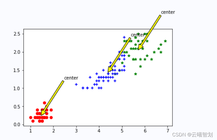
def draw(data,center,assment):
    length=len(center)
    fig=plt.figure
    data1=data[np.nonzero(assment[:,0].A == 0)[0]]
    data2=data[np.nonzero(assment[:,0].A == 1)[0]]
    data3=data[np.nonzero(assment[:,0].A == 2)[0]]
    # 选取前两个维度绘制原始数据的散点图
    plt.scatter(data1[:,0],data1[:,1],c="red",marker='o',label='label0')
    plt.scatter(data2[:,0],data2[:,1],c="green", marker='*', label='label1')
    plt.scatter(data3[:,0],data3[:,1],c="blue", marker='+', label='label2')
    # 绘制簇的质心点
    for i in range(length):
        plt.annotate('center',xy=(center[i,0],center[i,1]),xytext=\
        (center[i,0]+1,center[i,1]+1),arrowprops=dict(facecolor='yellow'))
        # plt.annotate('center',xy=(center[i,0],center[i,1]),xytext=\
        # (center[i,0]+1,center[i,1]+1),arrowprops=dict(facecolor='red'))
    plt.show()
    
    # 选取后两个维度绘制原始数据的散点图
    plt.scatter(data1[:,2],data1[:,3],c="red",marker='o',label='label0')
    plt.scatter(data2[:,2],data2[:,3],c="green", marker='*', label='label1')
    plt.scatter(data3[:,2],data3[:,3],c="blue", marker='+', label='label2')
    # 绘制簇的质心点
    for i in range(length):
        plt.annotate('center',xy=(center[i,2],center[i,3]),xytext=\
        (center[i,2]+1,center[i,3]+1),arrowprops=dict(facecolor='yellow'))
    plt.show()
    
    

dataSet = X
k = 3
centroids,clusterAssment = KMeans(dataSet,k)
draw(dataSet,centroids,clusterAssment)

输出结果如图3-2、3-3所示：

总结

The content of this series of articles is based on the first edition of Tsinghua University《机器学习实践》Relevant notes and insights made,The codes are all developed based on Baidu Feiye,If there is any infringement and inappropriateness,Please private message me,Actively cooperate with it,看到必回！！！

最后,A quote from this event,as the conclusion of the article～(￣▽￣～)~：

【学习的最大理由是想摆脱平庸,早一天就多一份人生的精彩;迟一天就多一天平庸的困扰.】