当前位置:网站首页>Data Mining-06
Data Mining-06
2022-08-09 13:41:00 【Draw a circle and curse you yebo】
maximum expectation
最大期望算法(Expectation-Maximization algorithm, EM),或Dempster-Laird-Rubin算法 ,is a kind of iterative极大似然估计(Maximum Likelihood Estimation, MLE)的优化算法 ,通常作为牛顿迭代法(Newton-Raphson method)Alternatives for the inclusion of latent variables(latent variable)or missing data(incomplete-data)的概率模型进行参数估计 .
EMThe standard computational framework of the algorithm is given byE步(Expectation-step)和M步(Maximization step)交替组成,The convergence of the algorithm ensures that the iterations at least approximate local maxima .EM算法是MM算法(Minorize-Maximization algorithm)one of the special cases of,There are multiple improved versions,包括使用了贝叶斯推断的EM算法、EM梯度算法、广义EM算法等.
Since iterative rules are easy to implement and flexibly consider hidden variables ,EMAlgorithms are widely used to deal with missing values in data,以及很多机器学习(machine learning)算法,包括高斯混合模型(Gaussian Mixture Model, GMM) 和隐马尔可夫模型(Hidden Markov Model, HMM) 的参数估计.
最大似然估计
The basic principle of maximum likelihood is actually very simple,Suppose we now have a sample in hand,This sample follows some distribution,while the distribution has parameters,But if I don't know what the specific parameters of this sample distribution are now,We want to analyze the sample obtained by sampling,In order to estimate a more accurate correlation parameter.
以上,This method of inversely inferring the distribution parameters through the sampling results is“最大似然估计”.Now simply think about how to estimate:A known distribution of the sampling results and the possible(比如说高斯分布),I like elementary equation,First set the parameters of the distribution(For example, the Gaussian distribution is setσσ和μμ),Then I calculate the probability function of the current sampled data,maximize this probability,See the value of relevant parameters.
这个思路很容易理解,The parameter that maximizes the probability must be“最可能”的那个,这里的“最可能”That is, in the maximum likelihood estimation“最大似然”的真正含义.
Just saying that might be a bit abstract,看一个具体的例子.The product is qualified、Not qualified,The unknown is the probability of nonconforming productpp,Obviously this is a typical distribution at two o 'clockb(1,p)b(1,p).We use random variablesXXIndicates whether it is qualified,X=0X=0表示合格,X=1X=1表示不合格.If you now get a set of sampled data(x1,x2,…,xn)(x1,x2,…,xn),Then it is not difficult to write the probability of sampling this set of data:
f(X1=x1,X2=x2,…,Xn=xn;p)=∏i=1npxi(1−p)1−xi
f(X1=x1,X2=x2,…,Xn=xn;p)=∏i=1npxi(1−p)1−xi
We call the above joint probability the likelihood function of the sample,Generally, take the logarithm of both sides of it at the same time(denoted as log-likelihood functionL(θ)L(θ)).L(θ)L(θ)关于ppThe partial derivative of,令偏导数为0,can be obtained such thatL(p)L(p)最大的pp值.
∂L(p)∂p=0⇒p^=∑i=1nxi/n
∂L(p)∂p=0⇒p^=∑i=1nxi/n
其中,求得的pp值称为pp的最大似然估计,to distinguish,用p^p^表示.
Other distribution may calculation process more complicated,However the basic steps are the same as this example.我们总结一下:Let the overall probability function bep(x;θ)p(x;θ),θθfor an unknown parameter,A sample from the population now knownx1,x2,…,xnx1,x2,…,xnthen ask forθθThe steps of maximum likelihood estimation of:
写出似然函数L(θ)L(θ),It is the joint probability function samples
L(θ)=p(x1;θ)⋅p(x2;θ)⋅…p(xn;θ)
L(θ)=p(x1;θ)⋅p(x2;θ)⋅…p(xn;θ)
take the logarithm of the likelihood function,并整理
ln(L(θ))=lnp(x1;θ)+⋯+lnp(xn;θ)
ln(L(θ))=lnp(x1;θ)+⋯+lnp(xn;θ)
关于参数θθ求偏导,并令偏导数为0,Solution to parameterθ^θ^,这就是参数θθ的最大似然估计
∂L(θ)∂θ=0⇒θ^=…
隐藏变量
Maximum Likelihood Estimation was introduced above,But the above approach is only applicable to probability models without hidden variables.What is a hidden variable,我们看这样一个例子.Suppose there are several male and female students in the class.,The heights of the students are subject to a normal distribution,当然了,The parameters of the height distribution of boys are different from the parameters of the height distribution of girls.Now if I give you the height of a classmate,It is very difficult to determine the classmate is male or female.If a sample is drawn at this time,Let you do the maximum likelihood estimation above,You will need to do the following two step operation:
Estimate whether each classmate in the sample is a boy or a girl;
Parameters for estimating the height distribution of boys and girls;
The second step is the maximum likelihood estimation mentioned above.,The difficulty is the first step,You still have to guess male and female.in more abstract language,可以这样描述:Samples belonging to multiple classes are mixed,Different categories of samples have different parameters,The task now is to sample from the population,Then estimate the distribution parameters of each category from the sampled data.This description is called“in probabilistic models that rely on unobservable hidden variables,Finding Maximum Likelihood Estimates for Parameters”,The hidden variable here is the class of the sample(such as the male and female).这个时候EM算法就派上用场了.
The digitized likelihood function
Assumes that the logarithm likelihood function is as follows:
lnL(θ)=ln(p(x1;θ)⋅p(x2;θ)⋅⋯⋅p(xn;θ))=∑i=1nlnp(xi;θ)=∑i=1nln∑j=1mp(xi,z(j);θ)(1)
(1)lnL(θ)=ln(p(x1;θ)⋅p(x2;θ)⋅⋯⋅p(xn;θ))=∑i=1nlnp(xi;θ)=∑i=1nln∑j=1mp(xi,z(j);θ)
公式(1)It's actually two steps,The first step is the normal logarithmization of the likelihood function,The second step is to put eachp(xi;θ)p(xi;θ)With different categories of joint distribution probability and said.It can be understood that the sample is drawnxixi的概率为xixi属于类z(1)z(1)的概率,加上xixi属于类z(2)z(2)的概率,加上...一直加到xixi属于类z(m)z(m)的概率.
本质上讲,Our purpose is to request the formula(1)的最大值.但是你看,现在(1)There is a sum in the logarithmic term in,If you ask for guidance,是非常麻烦的,所以,The first thing that comes to our mind is the formula(1)化简,Transformation in the form.
为了方便推导,我们将xixi对zzThe distribution function ofQi(z)Qi(z)表示.那么对于Qi(z)Qi(z),It must satisfy the following conditions:
∑j=1mQi(z(j))=1, Qi(z(j))≥0
∑j=1mQi(z(j))=1, Qi(z(j))≥0
所以公式(1)can be simplified like this:
lnL(θ)=∑i=1nln∑zp(xi,z(j);θ)=∑i=1nln∑j=1mQi(z(j))p(xi,z(j);θ)Qi(z(j))≥∑i=1n∑j=1mQi(z(j))lnp(xi,z(j);θ)Qi(z(j))(2)
(2)lnL(θ)=∑i=1nln∑zp(xi,z(j);θ)=∑i=1nln∑j=1mQi(z(j))p(xi,z(j);θ)Qi(z(j))≥∑i=1n∑j=1mQi(z(j))lnp(xi,z(j);θ)Qi(z(j))
这里的公式(2)非常重要,almost the wholeEM算法的核心公式.可以看到,The simplification process actually consists of two steps,The first is simply toQi(z)Qi(z)嵌入,The second is based onln()ln()The function is the last one obtained by the properties of the convex function ≥≥ 的结果.关于凸函数,I will be in this article4.2detail in section.Look at this formula,我们发现,通过化简,It is a lower bound of likelihood function are obtained(记为J(z,Q)J(z,Q)):
J(z,Q)=∑i=1n∑j=1mQi(z(j))lnp(xi,z(j);θ)Qi(z(j))
J(z,Q)=∑i=1n∑j=1mQi(z(j))lnp(xi,z(j);θ)Qi(z(j))
这个J(z,Q)J(z,Q)其实就是变量p(xi,z(j);θ)Qi(z(j))p(xi,z(j);θ)Qi(z(j))的期望.Recall that the desired algorithm isE(X)=∑xp(x)E(X)=∑xp(x),这里Qi(z(j))Qi(z(j))equivalent to probability.
我们发现,J(z,Q)J(z,Q)is easier to guide(because it is a simple addition),But the problem now is that the derivation of the lower bound is useless,We need to take the derivative of the likelihood function.换个思路想想,Nether depends onp(xi,z(j);θ)p(xi,z(j);θ)和Qi(z(j))Qi(z(j)),If we can continuously improve the lower bound through these two values,make it continue to approximate the probability functionln L(θ)ln L(θ),在某种情况下,如果J(z,Q)=ln L(θ)J(z,Q)=ln L(θ),那就大功告成了.说到这,先暂停,Let's look at the definition and properties of convex functions.
EMAlgorithm's convergence is proved
But we have a question here,Will this repeated iteration necessarily converge??假定θ(t)θ(t)和θ(t+1)θ(t+1)为第tt轮和第t+1t+1轮迭代后的结果,l(θ(t))l(θ(t))和l(θ(t+1))l(θ(t+1))is the corresponding likelihood function.显然,如果l(θ(t))≤l(θ(t+1))l(θ(t))≤l(θ(t+1)),So with the increase of the number of iterations,Step by step, will eventually approximate maximum likelihood values.也就是说,Just prove the formula(6)成立即可.
l(θ(t))<l(θ(t+1))(6)
(6)l(θ(t))<l(θ(t+1))
证明:得到θ(t)θ(t)后,执行E步:
Qti(z(j))=p(z(j)|xi;θt)
Qit(z(j))=p(z(j)|xi;θt)
此时,
l(θ(t))=∑i=1n∑j=1mQi(z(j))lnp(xi,z(j);θt))Qi(z(j))
l(θ(t))=∑i=1n∑j=1mQi(z(j))lnp(xi,z(j);θt))Qi(z(j))
然后执行M步,求偏导为0,得到θ(t+1)θ(t+1),此时有公式(7)成立:
l(θ(t+1))≥∑i=1n∑j=1mQi(z(j))lnp(xi,z(j);θ(t+1)))Qi(z(j))≥∑i=1n∑j=1mQi(z(j))lnp(xi,z(j);θt))Qi(z(j))=l(θt)(7)
(7)l(θ(t+1))≥∑i=1n∑j=1mQi(z(j))lnp(xi,z(j);θ(t+1)))Qi(z(j))≥∑i=1n∑j=1mQi(z(j))lnp(xi,z(j);θt))Qi(z(j))=l(θt)
Just say the formula(7),第一步l(θ(t+1))≥∑ni=1∑mj=1Qi(z(j))lnp(xi,z(j);θ(t+1))Qi(z(j))l(θ(t+1))≥∑i=1n∑j=1mQi(z(j))lnp(xi,z(j);θ(t+1))Qi(z(j))is determined by the previous formula(2)决定的;
第二步 ≥∑ni=1∑mj=1Qi(z(j))lnp(xi,z(j);θt))Qi(z(j))≥∑i=1n∑j=1mQi(z(j))lnp(xi,z(j);θt))Qi(z(j))是M步的定义,M步中,将θtθt调整到θ(t+1)θ(t+1)is to make the likelihood functionl(θ(t+1))l(θ(t+1))最大化.
综上,我们证明了EM算法的收敛性.
import matplotlib as mpl
import matplotlib.pyplot as plt

import numpy as np

from sklearn import datasets
from sklearn.mixture import GaussianMixture
from sklearn.model_selection import StratifiedKFold

colors = ['navy', 'turquoise', 'darkorange']

def make_ellipses(gmm, ax):
    for n, color in enumerate(colors):
        if gmm.covariance_type == 'full':
            covariances = gmm.covariances_[n][:2, :2]
        elif gmm.covariance_type == 'tied':
            covariances = gmm.covariances_[:2, :2]
        elif gmm.covariance_type == 'diag':
            covariances = np.diag(gmm.covariances_[n][:2])
        elif gmm.covariance_type == 'spherical':
            covariances = np.eye(gmm.means_.shape[1]) * gmm.covariances_[n]
        v, w = np.linalg.eigh(covariances)
        u = w[0] / np.linalg.norm(w[0])
        angle = np.arctan2(u[1], u[0])
        angle = 180 * angle / np.pi  # convert to degrees
        v = 2. * np.sqrt(2.) * np.sqrt(v)
        ell = mpl.patches.Ellipse(gmm.means_[n, :2], v[0], v[1],
                                  180 + angle, color=color)
        ell.set_clip_box(ax.bbox)
        ell.set_alpha(0.5)
        ax.add_artist(ell)

iris = datasets.load_iris()

# Break up the dataset into non-overlapping training (75%)
# and testing (25%) sets.
skf = StratifiedKFold(n_splits=4)
# Only take the first fold.
train_index, test_index = next(iter(skf.split(iris.data, iris.target)))


X_train = iris.data[train_index]
y_train = iris.target[train_index]
X_test = iris.data[test_index]
y_test = iris.target[test_index]

n_classes = len(np.unique(y_train))

# Try GMMs using different types of covariances.
estimators = dict((cov_type, GaussianMixture(n_components=n_classes,
                   covariance_type=cov_type, max_iter=20, random_state=0))
                  for cov_type in ['spherical', 'diag', 'tied', 'full'])

n_estimators = len(estimators)

plt.figure(figsize=(3 * n_estimators // 2, 6))
plt.subplots_adjust(bottom=.01, top=0.95, hspace=.15, wspace=.05,
                    left=.01, right=.99)


for index, (name, estimator) in enumerate(estimators.items()):
    # Since we have class labels for the training data, we can
    # initialize the GMM parameters in a supervised manner.
    estimator.means_init = np.array([X_train[y_train == i].mean(axis=0)
                                    for i in range(n_classes)])

    # Train the other parameters using the EM algorithm.
    estimator.fit(X_train)

    h = plt.subplot(2, n_estimators // 2, index + 1)
    make_ellipses(estimator, h)

    for n, color in enumerate(colors):
        data = iris.data[iris.target == n]
        plt.scatter(data[:, 0], data[:, 1], s=0.8, color=color,
                    label=iris.target_names[n])
    # Plot the test data with crosses
    for n, color in enumerate(colors):
        data = X_test[y_test == n]
        plt.scatter(data[:, 0], data[:, 1], marker='x', color=color)

    y_train_pred = estimator.predict(X_train)
    train_accuracy = np.mean(y_train_pred.ravel() == y_train.ravel()) * 100
    plt.text(0.05, 0.9, 'Train accuracy: %.1f' % train_accuracy,
             transform=h.transAxes)

    y_test_pred = estimator.predict(X_test)
    test_accuracy = np.mean(y_test_pred.ravel() == y_test.ravel()) * 100
    plt.text(0.05, 0.8, 'Test accuracy: %.1f' % test_accuracy,
             transform=h.transAxes)

    plt.xticks(())
    plt.yticks(())
    plt.title(name)

plt.legend(scatterpoints=1, loc='lower right', prop=dict(size=12))
plt.show()
边栏推荐
猜你喜欢

How to upload local file trial version in binary mode in ABAP report

Flutter入门进阶之旅(五)Image Widget
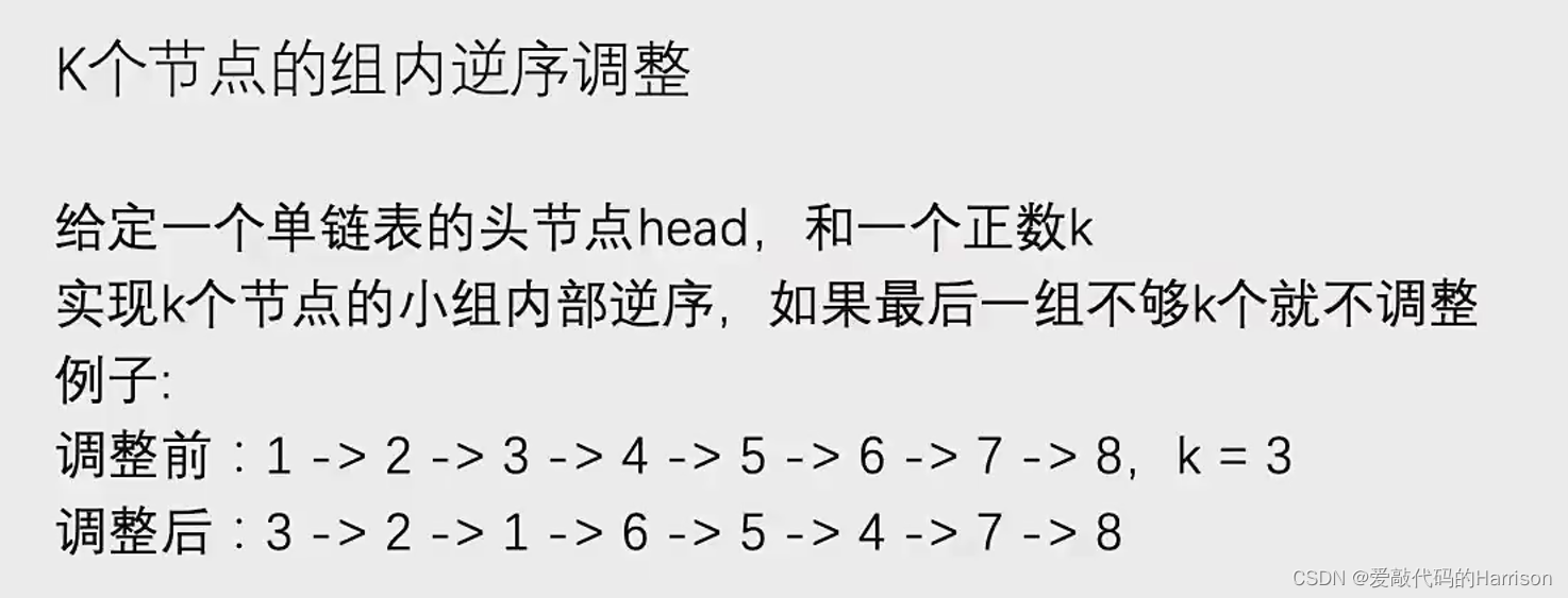
K个结点的组内逆序调整
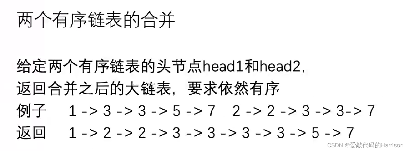
合并两个有序列表

Fragment中嵌套ViewPager数据空白页异常问题分析

Simple understanding of ThreadLocal
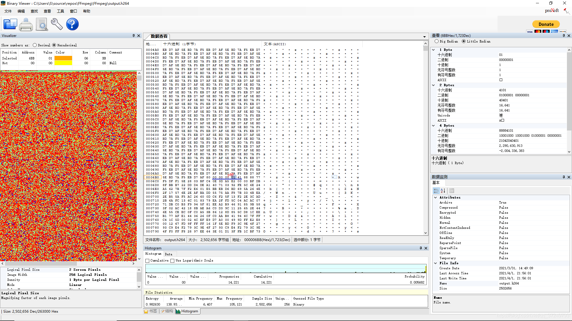
h264协议

Flutter入门进阶之旅(四)文本输入Widget TextField
史上最猛“员工”,疯狂吐槽亿万富翁老板小扎:那么有钱,还总穿着同样的衣服!...

又有大厂员工连续加班倒下/ 百度搜狗取消快照/ 马斯克生父不为他骄傲...今日更多新鲜事在此...
随机推荐
Flutter entry and advanced tour (6) Layout Widget
系统提供的堆 VS 手动改写堆
Flutter入门进阶之旅(七)GestureDetector
Go 事,如何成为一个Gopher ,并在7天找到 Go 语言相关工作,第1篇
合并两个有序列表
Flutter Getting Started and Advanced Tour (2) Hello Flutter
SQL Server查询优化 (转载非原创)
Redis源码剖析之robj(redisObject)
30行代码实现微信朋友圈自动点赞
ansible-cmdb友好展示ansible收集主机信息
Report: The number of students who want to learn AI has increased by 200%, and there are not enough teachers
随机快排时间复杂度是N平方?
世界第4疯狂的科学家,在103岁生日那天去世了
go基础之web获取参数
The FFmpeg library is configured and used on win10 (libx264 is not configured)
Flutter入门进阶之旅(八)Button Widget
Fragment中嵌套ViewPager数据空白页异常问题分析
【TKE】GR+VPC-CNI混用模式下未产品化功能配置
正则引擎的几种分类
位图与位运算