当前位置:网站首页>三、梯度下降求解最小θ
三、梯度下降求解最小θ
2022-04-23 14:37:00 【beyond谚语】
一、得到目标函数J(θ),求解使得J(θ)最小时的θ值
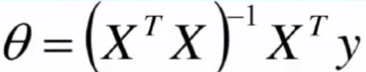
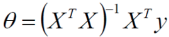
通过最小二乘法求目标函数最小值
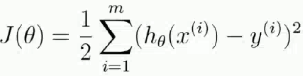
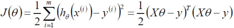
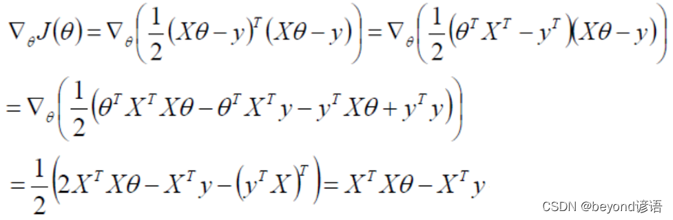
令偏导为0即可求解出最小的θ值,即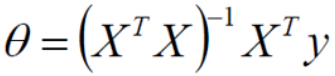
二、判定为凸函数
凸函数有需要判断方法,比如:定义、一阶条件、二阶条件等。利用正定性判定使用的是二阶条件。
半正定一定是凸函数,开口朝上,半正定一定有极小值
在用二阶条件进行判定的时候,需要得到Hessian矩阵,根据Hessian的正定性判定函数的凹凸性。比如Hessian矩阵半正定,函数为凸函数;Hessian矩阵正定,函数为严格凸函数
Hessian矩阵:黑塞矩阵(Hessian Matrix),又称为海森矩阵、海瑟矩阵、海塞矩阵等,是一个多元函数的二阶偏导数构成的方阵,描述了函数的局部曲率。
三、Hessian矩阵
黑塞矩阵是由目标函数在点x处的二阶偏导数组成的对称矩阵
正定:对A的特征值全为正数,那么A一定是正定的
不正当:非正定或半正定
若A的特征值≥0,则半正定,否则,A为非正定。
对J(θ)损失函数求二阶导,之后得到的一定是半正定的,因为自己和自己做点乘。
四、解析解
数值解是在一定条件下通过某种近似计算得出来的一个数值,能在给定的精度条件下满足方程,解析解为方程的解析式(比如求根公式之类的),是方程的精确解,能在任意精度下满足方程。
五、梯度下降法
这个课程跟其他课程讲的差不多,这里我就不再赘述了。梯度下降法
梯度下降法:是一种以最快的速度找到最优解的方法。
流程:
1,初始化θ,这里的θ是一组参数,初始化也就是random一下即可
2,求解梯度gradient
3,θ(t+1) = θ(t) - grand*learning_rate
这里的learning_rate常用α表示学习率,是个超参数,太大的话,步子太大容易来回震荡;太小的话,迭代次数很多,耗时。
4,grad < threshold时,迭代停止,收敛,其中threshold也是个超参数
超参数:需要用户传入的参数,若不传使用默认的参数。
六、代码实现
导包
import numpy as np
import matplotlib.pyplot as plt
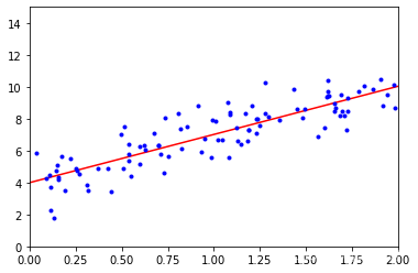
初始化样本数据
# 这里相当于是随机X维度X1,rand是随机均匀分布
X = 2 * np.random.rand(100, 1)
# 人为的设置真实的Y一列,np.random.randn(100, 1)是设置error,randn是标准正太分布
y = 4 + 3 * X + np.random.randn(100, 1)
# 整合X0和X1
X_b = np.c_[np.ones((100, 1)), X]
print(X_b)
""" [[1. 1.01134124] [1. 0.98400529] [1. 1.69201204] [1. 0.70020158] [1. 0.1160646 ] [1. 0.42502983] [1. 1.90699898] [1. 0.54715372] [1. 0.73002827] [1. 1.29651341] [1. 1.62559406] [1. 1.61745598] [1. 1.86701453] [1. 1.20449051] [1. 1.97722538] [1. 0.5063885 ] [1. 1.61769812] [1. 0.63034575] [1. 1.98271789] [1. 1.17275471] [1. 0.14718811] [1. 0.94934555] [1. 0.69871645] [1. 1.22897542] [1. 0.59516153] [1. 1.19071408] [1. 1.18316576] [1. 0.03684612] [1. 0.3147711 ] [1. 1.07570897] [1. 1.27796797] [1. 1.43159157] [1. 0.71388871] [1. 0.81642577] [1. 1.68275133] [1. 0.53735427] [1. 1.44912342] [1. 0.10624546] [1. 1.14697422] [1. 1.35930391] [1. 0.73655224] [1. 1.08512154] [1. 0.91499434] [1. 0.62176609] [1. 1.60077283] [1. 0.25995875] [1. 0.3119241 ] [1. 0.25099575] [1. 0.93227026] [1. 0.85510054] [1. 1.5681651 ] [1. 0.49828274] [1. 0.14520117] [1. 1.61801978] [1. 1.08275593] [1. 0.53545855] [1. 1.48276384] [1. 1.19092276] [1. 0.19209144] [1. 1.91535667] [1. 1.94012402] [1. 1.27952383] [1. 1.23557691] [1. 0.9941706 ] [1. 1.04642378] [1. 1.02114013] [1. 1.13222297] [1. 0.5126448 ] [1. 1.22900735] [1. 1.49631537] [1. 0.82234995] [1. 1.24810189] [1. 0.67549922] [1. 1.72536141] [1. 0.15290908] [1. 0.17069838] [1. 0.27173192] [1. 0.09084242] [1. 0.13085313] [1. 1.72356775] [1. 1.65718819] [1. 1.7877667 ] [1. 1.70736708] [1. 0.8037657 ] [1. 0.5386607 ] [1. 0.59842584] [1. 0.4433115 ] [1. 0.11305317] [1. 0.15295053] [1. 1.81369029] [1. 1.72434082] [1. 1.08908323] [1. 1.65763828] [1. 0.75378952] [1. 1.61262625] [1. 0.37017158] [1. 1.12323188] [1. 0.22165802] [1. 1.69647343] [1. 1.66041812]] """
# 常规等式求解theta
theta_best = np.linalg.inv(X_b.T.dot(X_b)).dot(X_b.T).dot(y)
print(theta_best)
""" [[3.9942692 ] [3.01839793]] """
# 创建测试集里面的X1
X_new = np.array([[0], [2]])
X_new_b = np.c_[(np.ones((2, 1))), X_new]
print(X_new_b)
y_predict = X_new_b.dot(theta_best)
print(y_predict)
""" [[1. 0.] [1. 2.]] [[ 3.9942692 ] [10.03106506]] """
绘图
plt.plot(X_new, y_predict, 'r-')
plt.plot(X, y, 'b.')
plt.axis([0, 2, 0, 15])
plt.show()
七、完整代码
import numpy as np
import matplotlib.pyplot as plt

# 这里相当于是随机X维度X1,rand是随机均匀分布
X = 2 * np.random.rand(100, 1)
# 人为的设置真实的Y一列,np.random.randn(100, 1)是设置error,randn是标准正太分布
y = 4 + 3 * X + np.random.randn(100, 1)

# 整合X0和X1
X_b = np.c_[np.ones((100, 1)), X]
print(X_b)

# 常规等式求解theta
theta_best = np.linalg.inv(X_b.T.dot(X_b)).dot(X_b.T).dot(y)
print(theta_best)

# 创建测试集里面的X1
X_new = np.array([[0], [2]])
X_new_b = np.c_[(np.ones((2, 1))), X_new]
print(X_new_b)
y_predict = X_new_b.dot(theta_best)
print(y_predict)

#绘图
plt.plot(X_new, y_predict, 'r-')
plt.plot(X, y, 'b.')
plt.axis([0, 2, 0, 15])
plt.show()
版权声明
本文为[beyond谚语]所创,转载请带上原文链接,感谢
https://beyondyanyu.blog.csdn.net/article/details/124360870
边栏推荐
猜你喜欢
关于在vs中使用scanf不安全的问题

想要成为架构师?夯实基础最重要
On the insecurity of using scanf in VS
电子秤称重系统设计,HX711压力传感器,51单片机(Proteus仿真、C程序、原理图、论文等全套资料)
Parameter stack pressing problem of C language in structure parameter transmission
1 minute to understand the execution process and permanently master the for cycle (with for cycle cases)
AT89C52单片机的频率计(1HZ~20MHZ)设计,LCD1602显示,含仿真、原理图、PCB与代码等

【STC8G2K64S4】比较器介绍以及比较器掉电检测示例程序
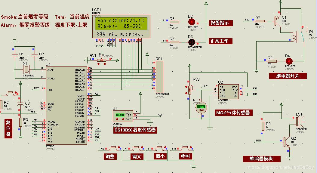
MQ-2和DS18B20的火灾温度-烟雾报警系统设计,51单片机,附仿真、C代码、原理图和PCB等
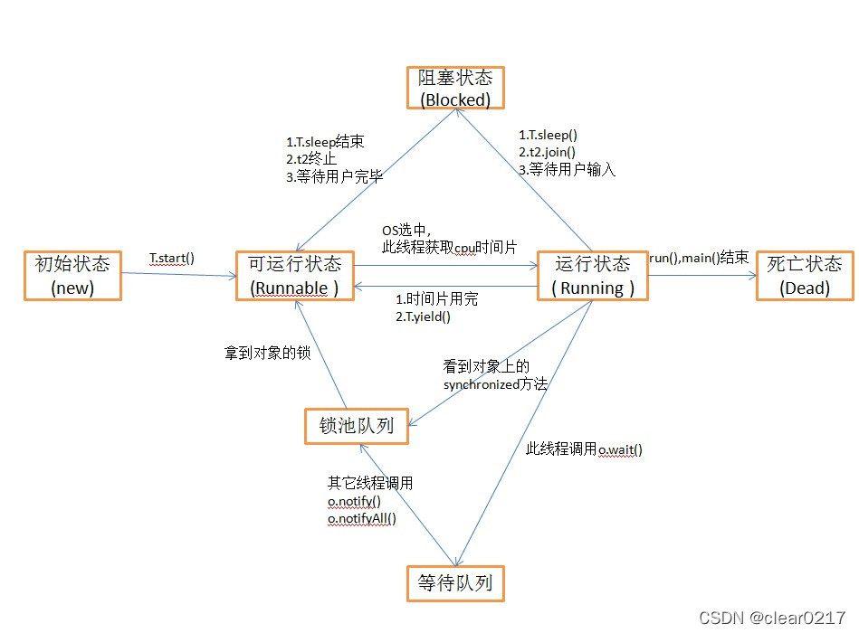
线程同步、生命周期
随机推荐
科技的成就(二十一)
初始c语言大致框架适合复习和初步认识
C语言知识点精细详解——初识C语言【1】——你不能不知的VS2022调试技巧及代码实操【2】
电容
爬虫练习题(一)
外包幹了四年,廢了...
C语言知识点精细详解——初识C语言【1】——你不能不知的VS2022调试技巧及代码实操【1】
Basic regular expression
GIS数据处理-cesium中模型位置设置
Design of single chip microcomputer Proteus for temperature and humidity monitoring and alarm system of SHT11 sensor (with simulation + paper + program, etc.)
async void 导致程序崩溃
QT actual combat: Yunxi calendar
C语言知识点精细详解——数据类型和变量【2】——整型变量与常量【1】
数组模拟队列进阶版本——环形队列(真正意义上的排队)
Achievements in science and Technology (21)
Swift - Literal,字面量协议,基本数据类型、dictionary/array之间的转换
《JVM系列》 第七章 -- 字节码执行引擎
初识STL
51 MCU + LCD12864 LCD Tetris game, proteus simulation, ad schematic diagram, code, thesis, etc
Golang 对分片 append 是否会共享数据