Pytorch Classical convolutional neural network LeNet

0. Introduction to the environment

Environment use Kaggle Built for free in Notebook

The tutorial uses Mr. Li Mu's Hands-on deep learning Website and Video Explanation

Tips ： When you don't understand the function, you can press Shift+Tab View function details .

1. LeNet

1.0 brief introduction

LeNet It is one of the earliest convolutional neural networks , Because of its efficient performance in computer vision tasks, it has attracted extensive attention . This model is made up of AT&T Researchers at Bell Labs Yann LeCun stay 1989 Put forward in （ And named after it ）, The purpose is to recognize the image [LeCun et al., 1998] Handwritten digits in . at that time ,Yann LeCun Published the first research on successfully training convolutional neural networks through back propagation , This work represents the achievements of neural network research and development in the past ten years .
at that time ,LeNet Achieved with support vector machine （support vector machines） Performance comparable results , Become the mainstream method of supervised learning . LeNet It is widely used in automatic teller machines （ATM） In flight , Help identify numbers that process checks . today , Some ATMs are still running Yann LeCun And his colleagues Leon Bottou In the last century 90 Code written in the era .
Address of thesis ：https://axon.cs.byu.edu/~martinez/classes/678/Papers/Convolution_nets.pdf

The handwritten digits MNIST Data sets ：

• $50,000$ Training data
• $10,000$ Test data
• Image size $28\times 28$
• $10$ class $(0\to 9)$

1.2 LeNet structure

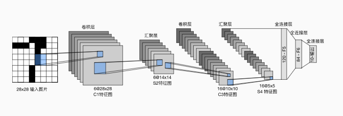
The basic unit in each convolution block is a convolution layer 、 One sigmoid Activation function and average pooling layer .
notes ： although ReLU Activating functions and maximizing pooling layers are more effective , But they are 20 century 90 The age has not yet appeared .

Each convolution layer uses $5\times 5$ Convolution kernel and a sigmoid Activation function . These layers map input to multiple 2D feature outputs , Usually increase the number of channels at the same time . The first convolution has $6$ Output channels , The second accretion layer has $16$ Output channels . Use $2\times 2$ The average pooling window reduces the dimension by spatial down sampling 4 times .

First use convolution layer to learn image spatial information , Then use the full connection layer to convert to category space .

2. Code implementation

2.1 Network structure

A small change has been made to the original model , Remove the Gaussian activation of the last layer . besides , This network is different from the original LeNet-5 Agreement .

!pip install -U d2l
import torch
from torch import nn
from d2l import torch as d2l

net = nn.Sequential(
    nn.Conv2d(1, 6, kernel_size=5, padding=2), nn.Sigmoid(),
    nn.AvgPool2d(kernel_size=2, stride=2),
    nn.Conv2d(6, 16, kernel_size=5), nn.Sigmoid(),
    nn.AvgPool2d(kernel_size=2, stride=2),
    nn.Flatten(),
    nn.Linear(16 * 5 * 5, 120), nn.Sigmoid(),
    nn.Linear(120, 84), nn.Sigmoid(),
    nn.Linear(84, 10))

X = torch.rand(size=(1, 1, 28, 28), dtype=torch.float32)
for layer in net:
    X = layer(X)
    print(layer.__class__.__name__,'output shape: \t',X.shape)

In the whole convolution block , Compared with the previous layer , The height and width of each layer feature are reduced . The first convolution layer uses $2$ Pixel fill , To compensate for the feature reduction caused by convolution kernel . The second accretion layer is not filled , Therefore, the height and width are reduced $4$ Pixel . As the stack rises , The number of channels varies from... At the time of input $1$ individual , Added after the first convolution layer $6$ individual , After the second accretion layer $16$ individual . meanwhile , The height and width of each average pool layer are halved . Last , Each fully connected layer reduces the dimension , Finally, an output whose dimension matches the number of result classifications is output .

2.2 load Fashion-MNIST Data sets

batch_size = 256
train_iter, test_iter = d2l.load_data_fashion_mnist(batch_size=batch_size)

2.3 Evaluation function

def evaluate_accuracy_gpu(net, data_iter, device=None): #@save
    """ Use GPU Calculate the accuracy of the model on the dataset """
    if isinstance(net, nn.Module):
        net.eval()  #  Set to evaluation mode 
        if not device:
            device = next(iter(net.parameters())).device
    #  The number of correct predictions , Total forecast quantity 
    metric = d2l.Accumulator(2)
    with torch.no_grad():
        for X, y in data_iter:
            if isinstance(X, list):
                # BERT Fine tuning required （ Then we will introduce ）
                X = [x.to(device) for x in X]
            else:
                X = X.to(device)
            y = y.to(device)
            metric.add(d2l.accuracy(net(X), y), y.numel())
    return metric[0] / metric[1]

2.4 Training functions

#@save
def train_ch6(net, train_iter, test_iter, num_epochs, lr, device):
    """ use GPU Training models ( Define in Chapter 6 )"""
    def init_weights(m):
        if type(m) == nn.Linear or type(m) == nn.Conv2d:
        	#  Use  xavier  Weight initialization 
            nn.init.xavier_uniform_(m.weight)
    net.apply(init_weights)
    print('training on', device)
    net.to(device)
    optimizer = torch.optim.SGD(net.parameters(), lr=lr)
    loss = nn.CrossEntropyLoss()
    animator = d2l.Animator(xlabel='epoch', xlim=[1, num_epochs],
                            legend=['train loss', 'train acc', 'test acc'])
    timer, num_batches = d2l.Timer(), len(train_iter)
    for epoch in range(num_epochs):
        #  The sum of training losses , The sum of training accuracy , Sample size 
        metric = d2l.Accumulator(3)
        net.train()
        for i, (X, y) in enumerate(train_iter):
            timer.start()
            optimizer.zero_grad()
            X, y = X.to(device), y.to(device)
            y_hat = net(X)
            l = loss(y_hat, y)
            l.backward()
            optimizer.step()
            with torch.no_grad():
                metric.add(l * X.shape[0], d2l.accuracy(y_hat, y), X.shape[0])
            timer.stop()
            train_l = metric[0] / metric[2]
            train_acc = metric[1] / metric[2]
            if (i + 1) % (num_batches // 5) == 0 or i == num_batches - 1:
                animator.add(epoch + (i + 1) / num_batches,
                             (train_l, train_acc, None))
        test_acc = evaluate_accuracy_gpu(net, test_iter)
        animator.add(epoch + 1, (None, None, test_acc))
    print(f'loss {
      train_l:.3f}, train acc {
      train_acc:.3f}, '
          f'test acc {
      test_acc:.3f}')
    print(f'{
      metric[2] * num_epochs / timer.sum():.1f} examples/sec '
          f'on {
      str(device)}')

2.5 use CPU Training

stay kaggle in Accelerator Set to None.

lr, num_epochs = 0.9, 10
train_ch6(net, train_iter, test_iter, num_epochs, lr, d2l.try_gpu())

Traversal per second $5612.2$ Samples .

2.6 use GPU Training

stay kaggle Use in GPU：

Traversal per second $33873.6$ Samples , It can be found that CPU Training is much faster .
Training set accuracy $0.820$, Test set accuracy $0.801$.

2.7 Try to change the activation function to ReLU And changing the pool layer to the maximum pool , Adjust the learning rate

net2 = nn.Sequential(
    nn.Conv2d(1, 6, kernel_size=5, padding=2), nn.ReLU(),
    nn.MaxPool2d(kernel_size=2, stride=2),
    nn.Conv2d(6, 16, kernel_size=5), nn.ReLU(),
    nn.MaxPool2d(kernel_size=2, stride=2),
    nn.Flatten(),
    nn.Linear(16 * 5 * 5, 120), nn.ReLU(),
    nn.Linear(120, 84), nn.ReLU(),
    nn.Linear(84, 10))

#  Learning rate  0.9  Will not converge when , So adjust it to  0.1
lr, num_epochs = 0.1, 10
train_ch6(net2, train_iter, test_iter, num_epochs, lr, d2l.try_gpu())

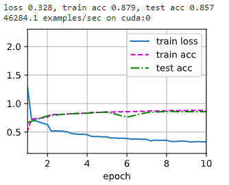
Training set accuracy $0.879$, Test set accuracy $0.857$, Compared with the previous model, it is indeed improved .