当前位置:网站首页>Lightweight network (1): MobileNet V1, V2, V3 series
Lightweight network (1): MobileNet V1, V2, V3 series
2022-08-11 08:45:00 【Tao Jiang】
轻量级网络(一):MobileNet V1,V2, V3系列
文章目录
在实际应用中,It's not just about the accuracy of the model,There is also a need to focus on the speed of the model.In consideration of both accuracy and speed,Lightweight networks came into being.Lightweight networks have performance comparable to bulky models,But compared to bulky models,有更少的参数和计算量,对硬件更友好.Lightweight network development so far,已经涌现了SqueezeNet系列,MobileNet系列,ShuffleNet系列,EfficientNet等等系列.This article is only for expositionMobileNet从V1到V3的发展历程.
MobileNet V1
MobileNet V1The main innovation of the version is the replacement of standard convolutions with depthwise separable convolutions.Depthwise separable convolutions are compared to standard convolutions,It can effectively reduce the amount of calculation and model parameters.如下表所示,Using depthwise separable convolutionsMobileNet,compared to using standard convolutionMobileNet,在ImageNetAccuracy on the dataset dropped1.1%,But the model parameters are reduced by approx7倍,The addition and multiplication calculations are reduced by approx9倍.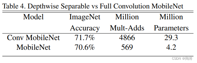
卷积计算量
标准卷积
Assume a standard convolutional input feature map F F F为 D F × D F × M D_{F} \times D_{F} \times M DF×DF×M,输出特征图 G G G为 D F × D F × N D_{F} \times D_{F} \times N DF×DF×N,其中是 D F D_{F} DF表示特征图的宽和高, M M M和 N N Nis the number of channels in the feature map.假设卷积核为 K K K,尺寸为 D K × D K × M × N D_{K} \times D_{K} \times M \times N DK×DK×M×N,其中 D K D_{K} DKare the kernel width and height.
Then a standard convolution operation,stride设为1,paddingMake the length and width of the output feature map the same as the input feature map,Then the calculation amount of standard convolution D K ⋅ D K ⋅ M ⋅ N ⋅ D F ⋅ D F D_{K} \cdot D_{K} \cdot M \cdot N \cdot D_{F} \cdot D_{F} DK⋅DK⋅M⋅N⋅DF⋅DF
深度可分卷积
深度可分卷积(depthwise separable convolution )is a form of decomposable convolution,It decomposes standard convolution into one**深度卷积(depthwise convolution)**和一个 1 × 1 1 \times 1 1×1卷积,其中 1 × 1 1 \times 1 1×1Convolution is calledpointwise convolution.深度卷积的filters尺寸大小为 D K × D K × 1 × M D_{K} \times D_{K} \times 1 \times M DK×DK×1×M,It applies a separate one on each input channelfliter,pointwise convolution利用 1 × 1 1 \times 1 1×1Convolution fuses the output channels of depthwise convolutions.这样分解,It can effectively reduce the amount of calculation and reduce the size of the model.
Suppose the input feature map of a depthwise separable convolution is D F × D F × M D_{F} \times D_{F} \times M DF×DF×M,Its output feature map is D F × D F × M D_{F} \times D_{F} \times M DF×DF×M,其中是 D F D_{F} DF表示特征图的宽和高, M M M和 N N Nis the number of channels in the feature map.
- 深度卷积: 卷积核为 D K × D K × 1 × M D_{K} \times D_{K} \times 1 \times M DK×DK×1×M,Then the output feature map size is D F × D F × M D_{F} \times D_{F} \times M DF×DF×M.
- 1*1卷积:卷积核为 1 × 1 × M × N 1 \times 1 \times M \times N 1×1×M×N,最后的输出为 D F × D F × M D_{F} \times D_{F} \times M DF×DF×M.
The computational cost of depthwise separable convolution is the sum of depthwise convolutionspointwise convolutionthe sum of the calculations,为 D K ⋅ D K ⋅ M ⋅ D F ⋅ D F + M ⋅ N ⋅ D F ⋅ D F D_{K} \cdot D_{K} \cdot M \cdot D_{F} \cdot D_{F} + M \cdot N \cdot D_{F} \cdot D_{F} DK⋅DK⋅M⋅DF⋅DF+M⋅N⋅DF⋅DF.
The following formula calculates the ratio of the computation amount of the depthwise separable convolution to the computation amount of the standard convolution,It can be seen that the depthwise separable convolution is a standard convolution 1 N + 1 D K 2 \frac{1}{N} + \frac{1}{D_{K}^{2}} N1+DK21.一般情况下,卷积核大小为 3 × 3 3 \times 3 3×3,为 D K 2 = 9 D_{K}^{2} = 9 DK2=9,卷积核的通道数 N N NThe value of is generally greater than 9,那么 1 N + 1 D K 2 > 1 9 \frac{1}{N} + \frac{1}{D_{K}^{2}} > \frac{1}{9} N1+DK21>91.
深度可分卷积 标准卷积 = D K ⋅ D K ⋅ M ⋅ D F ⋅ D F + M ⋅ N ⋅ D F ⋅ D F D K ⋅ D K ⋅ M ⋅ N ⋅ D F ⋅ D F = 1 N + 1 D K 2 \frac{深度可分卷积}{标准卷积}=\frac{D_{K} \cdot D_{K} \cdot M \cdot D_{F} \cdot D_{F} + M \cdot N \cdot D_{F} \cdot D_{F}}{D_{K} \cdot D_{K} \cdot M \cdot N \cdot D_{F} \cdot D_{F}}= \frac{1}{N} + \frac{1}{D_{K}^{2}} 标准卷积深度可分卷积=DK⋅DK⋅M⋅N⋅DF⋅DFDK⋅DK⋅M⋅DF⋅DF+M⋅N⋅DF⋅DF=N1+DK21
MobileNet V1The network architecture diagram is shown below: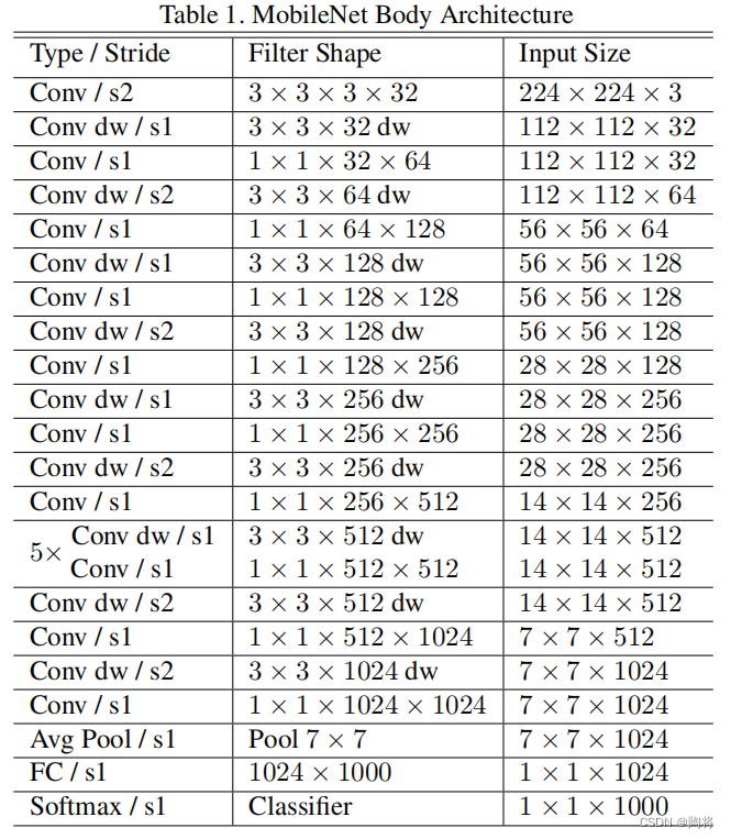
Model slimming down
From the comparison of the above-mentioned depthwise separable convolution and standard convolution,我们发现MobileNetThe architecture has fewer parameters and less computation than other convolutional network structures,But there are still many scenarios that require smaller and faster models.为了得到更小的模型,Two hyperparameters are introduced in the paper,宽度倍增器(width multiplier, α \alpha α)and a resolution multiplier(Resolution Multiplier, ρ \rho ρ),Slimming the model.The width multiplier acts on the number of channels per layer,The resolution multiplier works on the resolution size of the input image.
宽度倍增器
α \alpha α被称为宽度倍增器(width multiplier),The role is to slim down the network.对于某一层,Defines the width multiplier α \alpha α,Then enter the number of channels M M M则变成 α M \alpha M αM,输出通道数 N N N将变成 α N \alpha N αN. α ∈ ( 0 , 1 ] \alpha \in \left(0, 1 \right] α∈(0,1],一般取 1 , 0.75 , 0.5 , 0.25 1, 0.75, 0.5 , 0.25 1,0.75,0.5,0.25,当时 α = 1 \alpha =1 α=1是基础版MobileNet,当 α < 1 \alpha < 1 α<1is a shortened versionmobileNet.The amount of computation of the reduced depthwise separable convolution is shown in the following formula,The amount of computation is reduced α 2 \alpha^{2} α2倍.
D K ⋅ D K ⋅ α M ⋅ D F ⋅ D F + α M ⋅ α N ⋅ D F ⋅ D F D_{K} \cdot D_{K} \cdot \alpha M \cdot D_{F} \cdot D_{F} + \alpha M \cdot \alpha N \cdot D_{F} \cdot D_{F} DK⋅DK⋅αM⋅DF⋅DF+αM⋅αN⋅DF⋅DF
分辨率倍增器
ρ \rho ρis called a resolution multiplier(Resolution Multiplier),Input size increases/缩小 ρ \rho ρ倍,Then each layer in the network grows accordingly/缩小 ρ \rho ρ倍. ρ ∈ ( 0 , 1 ] \rho \in \left(0, 1 \right] ρ∈(0,1],The input resolution of the network is generally taken 224 , 192 , 160 , 128 224, 192, 160 , 128 224,192,160,128.当时 ρ = 1 \rho =1 ρ=1为基础版MobileNet,当 ρ < 1 \rho < 1 ρ<1is a shortened versionmobileNet.The amount of computation of the reduced depthwise separable convolution is shown in the following formula,It can be seen that the amount of calculation is reduced ρ 2 \rho^{2} ρ2倍.
D K ⋅ D K ⋅ α M ⋅ ρ D F ⋅ ρ D F + α M ⋅ α N ⋅ ρ D F ⋅ ρ D F D_{K} \cdot D_{K} \cdot \alpha M \cdot \rho D_{F} \cdot \rho D_{F} + \alpha M \cdot \alpha N \cdot \rho D_{F} \cdot \rho D_{F} DK⋅DK⋅αM⋅ρDF⋅ρDF+αM⋅αN⋅ρDF⋅ρDF
MobileNet V2
MobileNet V2 的创新点在于Inverse residual module with linear bottleneck( the inverted residual with linear bottleneck).在论文中,作者发现Using nonlinear functions in low-dimensional spaces loses some information,But in high dimensional space,The losses are relatively small.因此,引入Inverse residuals(Inverted Residuals)的概念,First increase the dimension and then do the convolution,Features are relatively well preserved.Increasing the dimension will increase the amount of calculation,因此需要降维,And because of nonlinearity, information will be lost,Therefore, dimensionality reduction is carried out in a linear way,is called a linear bottleneck(Linear Bottlenecks).
Bottleneck residual block
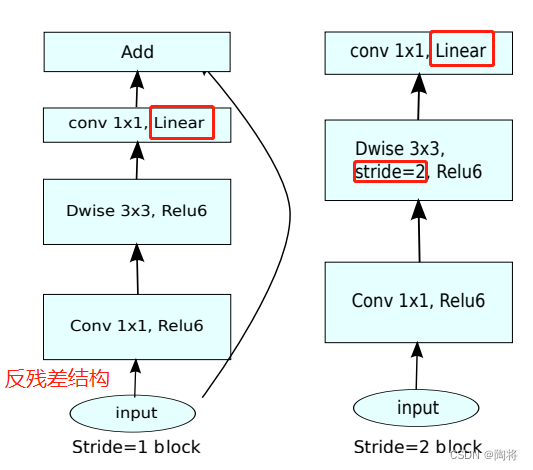
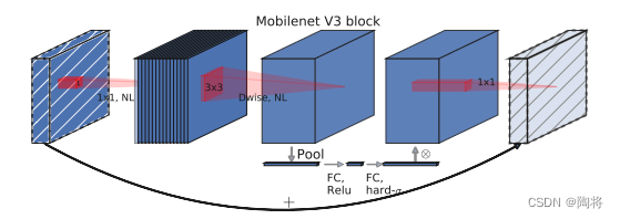
MobileNetV2和MobileNetV1相比,如上图所示,The depthwise convolutional sums are preserved 1 × 1 1 \times 1 1×1卷积,增加了 1 ∗ 1 1*1 1∗1Convolutional linear layer,MobileNet V2The base component is called Bottleneck residual block.不过 1 × 1 1 \times 1 1×1Convolution is after the input,Before depthwise convolution,The purpose is to expand the dimension.实验验证,使用 1 × 1 1 \times 1 1×1The purpose of linear convolution is to prevent nonlinearity from destroying too much information.strides为1时,Learn from the residual structure,However, it is different from the first decrease and then the increase of the number of channels in the residual structure,MobileNetV2The number of channels is increased first and then decreased.
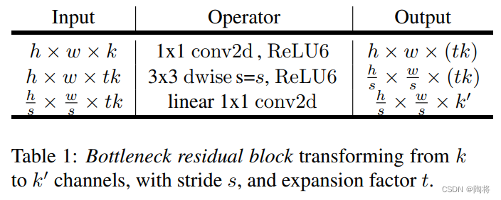
假设输入特征图大小为 h × w × k h \times w \times k h×w×k,首先经过一个 1 × 1 1 \times 1 1×1大小的卷积,输出特征图的大小为 h × w × ( t k ) h \times w \times \left(tk\right) h×w×(tk),其中 t t t是膨胀系数,MobileNet V2taken from the network architecture t = 6 t=6 t=6.followed by one 3 × 3 3 \times 3 3×3大小的卷积,步数为 s s s,输出特征图大小为 h s × w s × ( t k ) \frac{h}{s} \times \frac{w}{s} \times \left( tk \right) sh×sw×(tk),最后经过一个 1 × 1 1 \times 1 1×1A linear convolution of size,得到最后的输出,输出特征图大小为 h × w × k ′ h \times w \times {k}' h×w×k′.
模型架构
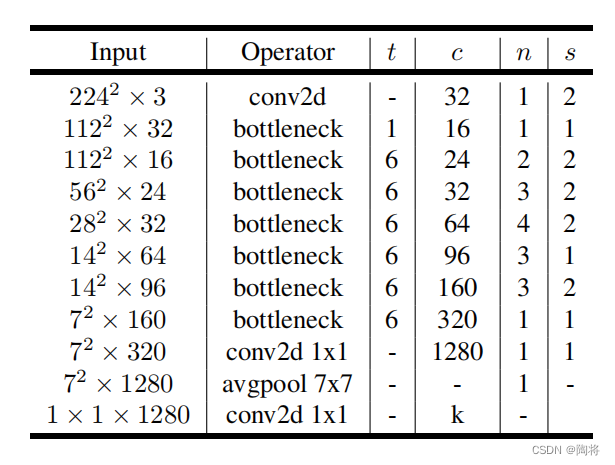
MobileNet V2的网络架构如下图所示,其实 t t t为膨胀系数, c c c是通道数, n n n是重复次数, s s s是步数.
MobileNet V3
MnasNet在MobileNet V2 Bottleneck block的基础上加入SEModules introduce lightweight attention,如上图所示,In order to apply attention to the maximum representation,SEThe module is used after the dilated depthwise separable convolution.MobileNet V3Included in the network architectureMnasNet和MobileNet V2基础块.
MobileNet V3The construction of the network architecture consists of two steps:首先,由platform-aware NAS和NetAdaptAlgorithm compound network search search basic architecture;Then several new components are introduced to improve model performance,形成最终模型.platform-aware NASSearch the global network structure by optimizing each network block,NetAdaptThe algorithm searches each layerfilter数量.MobileNet V3A new nonlinear function is introduced in ,h-swish(swish的改进版),It's capable of faster stages,And quantification is more friendly.MobileNet V3 under the premise of maintaining accuracy,Redesigned computationally expensive network start and end layers,减少延迟.See this paper for details.
s w i s h x = x ⋅ σ ( x ) h − s w i s h [ x ] = s R e L U 6 ( x + 3 ) 6 swish \; x = x \cdot \sigma \left( x \right) \\ h-swish\left[ x \right] = s \frac{ReLU6\left( x + 3 \right)}{6} swishx=x⋅σ(x)h−swish[x]=s6ReLU6(x+3)
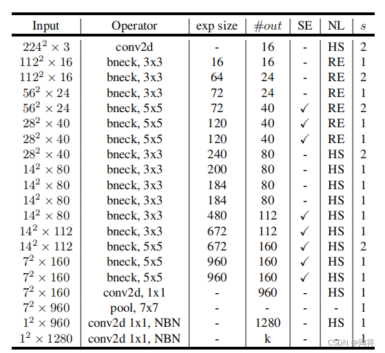
MobileNet V3有两个模型:MobileNetV3-Large 和 MobileNetV3-Small.The network structure of the large and small models is shown in the following table,They target high and low resource use cases, respectively.其中SE表示在block中是否包括Squee-And-Excite.NLis a nonlinear type,其中HS表示h-swish,RE表示ReLU.NBN表示没有BN操作.
MobileNetV3-Large网络结构如下所示:
MobileNet V3 small网络结构如下所示: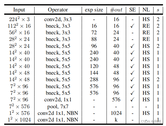
MobileNet V1,V2,V3对比
以下是MobileNetV1-V3The networks are thereImageNet-1k上的top-1Accuracy and parameters are compared.
| Network | Top-p1 | Params |
|---|---|---|
| MobileNetV1 | 70.6 | 4.2M |
| MobileNetV2 | 72.0 | 3.4M |
| MobileNetV2(1.4) | 74.7 | 6.9M |
| MobileNetV3-Large(1.0) | 75.2 | 5.4M |
| MobileNetV3-Large(0.75) | 73.3 | 4.0M |
| MobileNetV3-Small(1.0) | 67.4 | 2.5M |
| MobileNetV3-Small(0.75) | 65.4 | 2.0M |
参考
边栏推荐
猜你喜欢
SDUT 2877: angry_birds_again_and_again
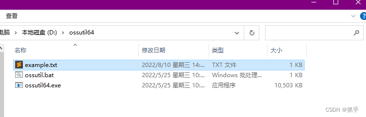
阿里云OSS上传文件超时 探测工具排查方法
基于C#通过PLCSIM ADV仿真软件实现与西门子1500PLC的S7通信方法演示

关于架构的认知
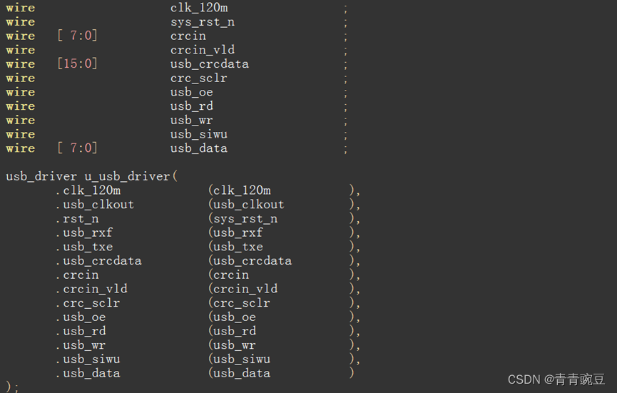
FPGA 20个例程篇:11.USB2.0接收并回复CRC16位校验
【wxGlade学习】wxGlade环境配置
C语言操作符详解
Alibaba Sentinel - Slot chain解析
go-grpc TSL authentication solution transport: authentication handshake failed: x509 certificate relies on ... ...
对比学习系列(三)-----SimCLR
随机推荐
WiFi cfg80211
magical_spider远程采集方案
IDEA的初步使用
flex布局回顾
【415. 字符串相加】
基于 VIVADO 的 AM 调制解调(1)方案设计
场地预订系统,帮助场馆提高坪效
Break pad source code compilation--refer to the summary of the big blogger
Getting Started with Kotlin Algorithm to Calculate the Number of Daffodils
YTU 2297: KMP pattern matching three (string)
Nuget找不到包的问题处理
基于C#通过PLCSIM ADV仿真软件实现与西门子1500PLC的S7通信方法演示
excel将数据按某一列值分组并绘制分组折线图
pycharm中绘图,显示不了figure窗口的问题
opengauss创建用户权限问题
选择收银系统主要看哪些方面?
程序员是一碗青春饭吗?
go 操作MySQL之mysql包
One network cable to transfer files between two computers
Linux,Redis中IOException: 远程主机强迫关闭了一个现有的连接。解决方法