Address of thesis ：https://arxiv.org/abs/2112.08177
Source code address ：https://github.com/baegwangbin/MaGNet

---

summary

starting point ：

• MVS Building multi view matching cost body brings huge video memory consumption
• Monocular depth estimation in the absence of （ weak ） Texture area 、 Reflective surface 、 The estimation effect in the case of moving objects is better than
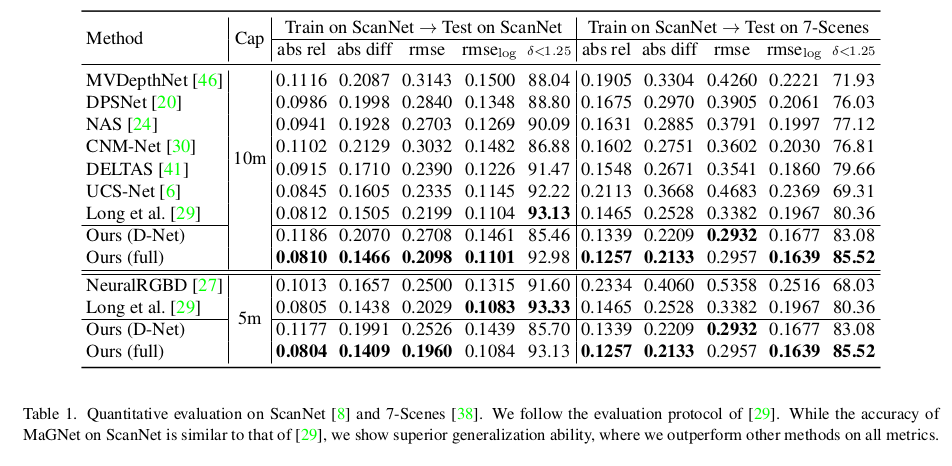
     So , In this paper, a new framework combining single view depth probability and multi view geometry is proposed (Monocular and Geometric Network : MaGNet), For each frame of image ,MaGNet Predict the depth probability distribution of single view , It is parameterized into a Gaussian distribution at the pixel level ; then , The distribution estimated by the reference frame is used to sample the prime depth assumption . This probabilistic sampling strategy enables the network to establish fewer depth assumptions and obtain higher accuracy ; The depth consistency weighting method is also proposed for the multi view matching score , To ensure that the multi view depth is consistent with the single view prediction .
  The innovations of the article are as follows ：
• Probabilistic depth sampling（ Depth value sampling based on probability distribution ）： The probability distribution is obtained from monocular estimation , Use probability distribution to generate depth assumptions ;
• Depth consistency weighting for multi-view matching（ Multi view depth consistency weight ）： The depth probability distribution of single view is used to generate multi view matching weight , The multi view matching results are weighted ;
• Iterative refinement（ Iterative optimization strategy ）： A compact initial matching cost volume is constructed by using the depth hypothesis volume constructed by probability distribution and multi view consistency weight , If there is an error in the depth probability distribution of a single view , As a result, the depth assumption cannot be obtained by sampling . In view of this situation, a strategy based on iterative optimization is proposed , The updated probability distribution is fed back to the probability depth sampling module , Continuously improve the accuracy of probability distribution ;

It mainly includes the following steps ：

1. Predict the depth probability distribution of a single frame image , And parameterize it into Gaussian distribution ;
2. The predicted distribution is used to sample the depth of each pixel of the reference image to obtain the depth assumption value ;
3. Using depth assumptions and camera parameters, the features of the reference frame are extracted warp To neighborhood frame , The matching cost is calculated by point multiplication ;
4. The matching score of each adjacent view is multiplied by the binary depth consistency weight inferred from the single view depth probability estimated by the view ;
5. Using the matching cost volume, the matching probability volume is obtained by cost volume regularization ;
6. step 2-5 Iterations can be repeated to improve accuracy ;

In this way , The final output is the pixel by pixel depth probability distribution , From this, we can infer the expected value and related uncertainty .

---

Model architecture

   The goal of the model is to predict the reference frame $I_t$ stay t Depth map of time , Input as pictures in a time series ： W t = { I t − 2 Δ t , I t − Δ t , I t , I t + Δ t , I t + 2 Δ t } \mathcal{W}_{t}=\left\{I_{t-2 \Delta t}, I_{t-\Delta t}, I_{t}, I_{t+\Delta t}, I_{t+2 \Delta t}\right\} Wt​={ It−2Δt​,It−Δt​,It​,It+Δt​,It+2Δt​} And camera parameters , Pictured 2 Shown , It mainly includes the following 3 A step ：1. Feature extraction and depth probability distribution prediction are carried out for each frame image ;2. The depth hypothesis is sampled through probability distribution , And generate multi view consistency weights ;3. The matching cost volume is used to estimate the multi view depth probability volume ;

Single-View Depth Probability and Features（ Single view feature extraction and depth probability distribution construction ）

Single-view depth probability

   about ${\mathcal{W}}_t\in R^{H\times W}$ Each input image in $I_t$, Use D-Net To predict its depth probability distribution $\in R^{\frac{H}{4}\times \frac{W}{4}}$, about $I_t$ Every pixel $(u,v)$ , The probability distribution is parameterized as follows 1 Shown ：
$$p_{u,v}\left(d\mid I_t\right)=\frac{1}{{\sigma }_{u,v}\left(I_t\right)\sqrt{2\pi }}{e}^{-\frac{1}{2}{\left(\frac{d-{\mu }_{u,v}\left(I_t\right)}{{\sigma }_{u,v}\left(I_t\right)}\right)}^2}\text{\hspace{1em}(1)}$$
among $\mu and\sigma$ Is the mean and variance , A lightweight codec structure and EfficientNet B5 As a backbone network , The linear activation layer is used to calculate the mean value $\mu$ , Use modified ELU Function to calculate the variance $\sigma$ ：$f(x)=ELU(x)+1$, This ensures that the calculated variance is positive , And has a smooth gradient ; When training the rest of the modules, you need to D-Net The weights are frozen ; Use NLL Loss to monitor model training ：
$$L_{u,v}\left(d_{u,v}^{\mathrm{g}\mathrm{t}}\mid I_t\right)=\frac{1}{2}\log {\sigma }_{u,v}^2\left(I_t\right)+\frac{{\left(d_{u,v}^{\mathrm{g}\mathrm{t}}-{\mu }_{u,v}\left(I_t\right)\right)}^2}{2{\sigma }_{u,v}^2\left(I_t\right)}\text{\hspace{1em}(2)}$$
The above formula means , At the boundary point of the object , When the model is difficult to reduce $(d^{gt}-\mu {)}^2$ The error of the , Will make the standard deviation ${\sigma }^2$ Larger to make the second term smaller , The first will limit the variance to too large ; In non boundary areas , At this time, the correct depth value is different from the estimated depth value $\mu$ Close , The second term is approximately 0, In order to make the whole loss function smaller , The model tends to make the first term smaller , That is to say ${\sigma }^2$ smaller ;

Single-view features

   Use F-Net To extract the features of each picture $\in R^{\frac{H}{4}\times \frac{W}{4}}$, Then the matching cost volume is calculated based on the point multiplication of the corresponding point eigenvector , For pixels $(u,v)$ At depth { d k } k = 1 N s \{d_k\}_{k=1}^{N_s} { dk​}k=1Ns​​, The matching cost is as follows 3 Shown ：
$$s_{u,v,k}\left(I_t\right)=\sum _{i\ne t}*{\mathbf{f}}_{u,v}\left(I_t\right),{\mathbf{f}}_{u_{ik},v_{ik}}\left(I_i\right)*\text{\hspace{1em}(3)}$$

   stay depth Dimensionality softmax Get the probability body $p_{u,v,k}=sofrma{x}_k(s_{u,v,k})$, Finally, the depth map is calculated based on the expectation ${\hat{d}}_{u,v}={\sum }_k{p}_{u,v,k}\cdot d_k$,F-Net By uniformly sampling the depth of the assumed volume { d k } \{d_k\} { dk​} And minimize $\widehat{d_{u,v}}And{d}_{u,v}^{gt}$ Between L1 Get the pre training weight ;

Fusing Single-View Depth Probability with Multi-View Geometry（ Single view depth probability distribution and multi view geometric information fusion ）

notes : This process has no parameters to learn （ No gradient descent is required ）

Probabilistic depth sampling( Depth hypothesis sampling based on probability distribution )

   In this paper, the depth assumption value of each pixel is defined, and the search range is $[{\mu }_{u,v}-\beta {\sigma }_{u,v},{\mu }_{u,v}+\beta {\sigma }_{u,v}]$, KaTeX parse error: Undefined control sequence: \bata at position 1: \̲b̲a̲t̲a̲ For a super parameter , Then divide the search scope into 10 Intervals , This allows more depth assumptions to approach ${\mu }_{u,v}$ , The midpoint of each interval is the assumed value of depth , The first k A depth assumption $d_{u,v,k}$ The definition is as follows 4 Shown ：
$$\begin{gathered} d_{u,v,k}={\mu }_{u,v}+b_k{\sigma }_{u,v} \\ where\begin{array}{rlr}{b}_k=\frac{1}{2}[& {\Phi }^{-1}\left(\frac{k-1}{N_s}{P}^{\ast }+\frac{1-P^{\ast }}{2}\right)& +{\Phi }^{-1}\left(\frac{k}{N_s}{P}^{\ast }+\frac{1-P^{\ast }}{2}\right)]\end{array}\text{\hspace{1em}(4)} \end{gathered}$$
among ,${\Phi }^{-1}(.)$ It's a probability function , and $P^{\star }=erf(\beta /\sqrt{2})$ Indicates the interval $[{\mu }_{u,v}-\beta {\sigma }_{u,v},{\mu }_{u,v}+\beta {\sigma }_{u,v}]$ The probability mass of ;
notes ： { b k } \{b_k\} { bk​} Only with $N_s$ and $\beta$ of , There is no need to calculate per pixel ;

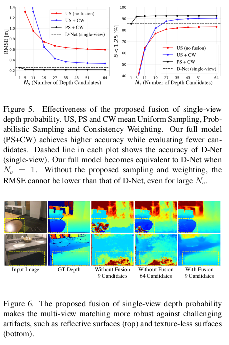
chart 3 The left side compares the uniform sampling with the sampling method proposed in this paper , For pixels with high uncertainty , Increase the spacing between candidate points , Thus, a wider range of candidate points can be evaluated .

Depth consistency weighting( Depth consistency weight )

   If the depth assumption is correct , Explain the corresponding 3D The point is on the surface of the object , If this 3D The point is visible in the neighborhood view , Then the probability value of the corresponding single view to this depth should be high ; Equivalent to “ If the single view depth probability of the depth assumption estimated from adjacent views is low , It means that the depth candidate is wrong or it is not visible in the view （ For example, due to occlusion ）”; So , The score of multi view matching is as follows 5 Shown ：
$$\begin{array}{rl}{s}_{u,v,k}\left(I_t\right)& =\sum _{i\ne t}{w}_{u_{ik},v_{ik},d_{ik}}^{\mathrm{d}\mathrm{c}}*{\mathbf{f}}_{u,v}\left(I_t\right),{\mathbf{f}}_{u_{ik},v_{ik}}\left(I_i\right)*\\ & \\ w_{u_{ik},v_{ik},d_{ik}}^{\mathrm{d}\mathrm{c}}& =\delta \left(p_{u_{ik},v_{ik}}\left(d_{ik}\mid I_i\right)>p_{\text{thres }}\right)\end{array}\text{\hspace{1em}(5)}$$
among , When the depth probability of single view $p_{u_{ik},v_{ik}}\left(d_{ik}\mid I_i\right)>p_{\text{thres }}$ when , $w_{u_{ik},v_{ik},d_{ik}}^{\mathrm{d}\mathrm{c}}=1$ , Or equal to 0, take $s_{u,v,k}\left(I_t\right)$ As the depth consistency weight ;$p_{\text{thres }}$ The setting of is very important , Too many candidate depth values will be eliminated （ It may contain the correct depth value ）; Set in the text $p_{\text{thres }}=\exp \left(-{\kappa }^2/2\right)/{\sigma }_{u_{ik},v_{ik}}\sqrt{2\pi }$, If $d_{i,k}$ stay k-sigma Within the confidence interval of p Will tend to 1,$p_{\text{thres }}$ Is determined by each pixel and the view ; If D-Net Uncertainty about the predicted depth （$\sigma$ It's big ）, be $p_{thres}$ Very low , More depth assumptions can be considered ;
   Depth consistency weighting can eliminate candidate depth values with low single view depth probability . Especially when the multi view matching is not clear or reliable , This weighting method can improve the robustness of the model . for example , If the pixel is within a textured surface , A wide range of depth candidates will result in similar matching scores . If the scene contains reflective surfaces , The matching score is calculated between reflections , This leads to overestimation of depth . In both cases ,MaGNet Both can make robust prediction by favoring depth candidates with high single view depth probability .

Estimating Multi-View Depth Probability Distribution ( Multi view depth probability distribution estimation )

Updating single-view depth probability distribution( Update the single view depth probability distribution )

   Thanks to the depth hypothesis sampling strategy based on probability distribution , The dimension of the matching cost obtained by the model is $\frac{H}{4}\times \frac{W}{4}\times N_s$ , among $N_s$ Is the number of depth assumptions ; Enter it as , Use G-Net Update the mean and variance of single view to estimate the multi view depth probability distribution ; because ${\mu }_{u,v}$ and ${\sigma }_{u,v}$ Not coded in input , It is difficult to update the mean and variance of by direct regression . So ,G-Net Adopt the idea of residual learning , Estimate the normalized residual value of mean and variance $\Delta {\mu }_{u,v}/{\sigma }_{u,v}$. For example, when the parallax of two pixels is $k^{\prime }$ When the match score is high , Model to learn $b_{k^{\prime }}$ To update the mean ：${\mu }_{u,v}^{\text{new }}={\mu }_{u,v}+b_{k^{\prime }}{\sigma }_{u,v}$. Empathy ,G-Net Study ${\sigma }_{u,v}^{\text{new }}/{\sigma }_{u,v}$ To update the variance value ; In this way, the depth probability distribution of multi view is updated ; notes ：G-Net The output of can be fed back to the sampling module , And the process can be repeated to continuously optimize the output .

Learned upsampling( Learnable upsampling )

  G-Net The output of is a multi view probability distribution diagram $\in R^{2\times \frac{H}{4}\times \frac{W}{4}}$, In order to sample this probability distribution map to the original resolution , In this paper, a learning up sampling strategy is proposed ： The input to the model is D-Net Characteristic graph , Use a lightweight CNN To predict the $R^{1\times (3\ast 3)\times 4\times 4\times \frac{H}{4}\times \frac{W}{4})}$ Of mask (4 Represents the scale of the original image ) , Plot the probability distribution $R^{2\times \frac{H}{4}\times \frac{W}{4}}$ Every point of $3\times 3$ Take out the neighborhood pixels of , Form neighborhood characteristic graph $\in R^{2\times (3\ast 3)\times 1\times 1\times \frac{H}{4}\times \frac{W}{4}}$ , With the mask After dot multiplication, it will be in $3\ast 3$ Sum the dimensions to get $R^{2\times 4\times 4\times \frac{H}{4}\times \frac{W}{4}}$ , Last resize obtain $R^{2\times H\times W}$

def upsample_depth_via_mask(depth, up_mask, k):
    # depth: low-resolution depth (B, 2, H, W)
    # up_mask: (B, 9*k*k, H, W)
    N, o_dim, H, W = depth.shape
    up_mask = up_mask.view(N, 1, 9, k, k, H, W)
    up_mask = torch.softmax(up_mask, dim=2)             # (B, 1, 3*3, k, k, H, W)

    up_depth = F.unfold(depth, [3, 3], padding=1)       # (B, 2, H, W) -> (B, 2 X 3*3, H*W)
    up_depth = up_depth.view(N, o_dim, 9, 1, 1, H, W)   # (B, 2, 3*3, 1, 1, H, W)
    up_depth = torch.sum(up_mask * up_depth, dim=2)     # (B, 2, k, k, H, W)

    up_depth = up_depth.permute(0, 1, 4, 2, 5, 3)       # (B, 2, H, k, W, k)
    return up_depth.reshape(N, o_dim, k*H, k*W)         # (B, 2, k*H, k*W)

Iterative refinement and network training( Iterative optimization and model training )

   Through repeated iterations $N_{iter}$ Multiple view matching process （ Depth hypothesis sampling based on probability distribution ——> Multi view consistency weight matching ——> adopt G-Net Update the probability distribution parameters ） You can get $N_{iter}$ A prediction ; Calculate the formula in each iteration 2 Of NLL Loss , Calculated by each iteration NLL The loss is multiplied by ${\gamma }^{N_{\text{iter }}-i}$ ( The weight of the back is greater than that of the front ), The sum of these losses is used to train G-Net With a learnable mountain sampling module ;
   This iterative strategy has two benefits ： (1) If in an iteration , The matching score of a pixel is high , Then the mean value of the depth hypothesis space will converge to the predicted depth value of the pixel and the variance will decrease , In the next iteration, we will look for the depth hypothesis space near the last maximum value , This can lead to higher matching scores ;(2) Iterative updates can also prevent D-Net Inaccurate prediction leads to model collapse , For example, the of a pixel Ground True The search scope of the initial depth assumption space is no longer $[{\mu }_{u,v}-\beta {\sigma }_{u,v},{\mu }_{u,v}+\beta {\sigma }_{u,v}]$ Inside , No candidate depth value can get a high matching score , In this case G-Net Will be reduced by 2 Of NLL Loss value to get a larger variance value , In the next iteration, we can find the depth value in a wider range ;

---

experimental result