Random neurons and random depth of dropout Technology

1. Write it at the front

Learning to reproduce EfficientNet When it comes to the Internet , There's a MBConv The module looks like this ：

Of course , The structure itself is not very novel , from resNet Start , Almost a lot of networks behind , such as DenseNet, MobileNet series ,ShuffleNet Series and EfficientNet The series will find such a residual structure . But this exploration found Dropout This point , Previously, when implementing the residual structure , If you come across Dropout, I always thought it was the random inactivation of neurons learned before Dropout, But I didn't find it until I saw the source code here , It's not as simple as I thought ！

This residual structure is used in Dropout, It's called random depth Dropout technology . This is 2016 year ECCV An article published in paper, The paper is called 《Deep Network with Stochastic depth》, It's about training , Instead of randomly inactivating neurons in each layer , Instead of randomly removing many layers , This reduces redundancy , It can also speed up training .

out of curiosity , I read this article paper, Also learned a kind of training operation with residual network , therefore , This article wants to unify the two Dropout Put a piece to tidy up .

2. Dropout Random neurons

This technology is common Dropout Technology ,Dropout Random inactivation of neurons , Is that we give a probability , Let the weight of a neuron in the neural network layer be 0( Deactivation )

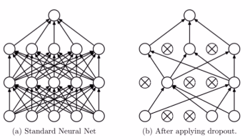
It's every floor , Make some neurons inoperative , This is equivalent to simplifying the network ( The left and right can be compared ）, We sometimes appear Over fitting phenomenon , Because our network is too complex , Too many parameters , And our network in the back layer may be too dependent on a neuron in the front layer .

Join in Dropout after , First, the network will become simple , Reduce some parameters , And because we don't know which neurons in the shallow layer will be inactivated , As a result, the back network dare not put too much weight on a neuron in the front layer , This reduces a phenomenon of excessive dependence , Less dependence on features , thus It is beneficial to alleviate over fitting .

Is this similar to our final exam , The teacher always draws a key point for us , But because we don't know which of these key points will really appear on the test paper , So we have to divide our energy evenly , Have to see , It's safer , Can also generalize a little , At least as long as these types of questions can be done . And if we don't divide our energy evenly , Focus only on certain types of questions , Then it must be a wave

So this kind of Dropout Technology can help the network alleviate over fitting . Not too hard to understand , But there are several precautions when using ：

1. Data scale changes
   We use it Dropout It's used like this when ： Only turn it on during training Dropout, When testing, you don't have to Dropout Of , In other words, some neurons will be inactivated randomly during model training , And when we test, we use all the neurons , Then the problem of data scale will arise at this time , So when it comes to testing , The weight of ownership is multiplied by 1-drop_prob, To ensure that the scale changes during training and testing are consistent . How to understand ？ Still take the picture above ：
   
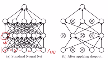
   Suppose our input is 100 Features , So the expression of the first neuron in the first layer should be like this , Let's assume that there is no inactivation ：
   $$Z_1^1=\sum _{i=1}^{100}{w}_i{x}_i$$
   Suppose we have $w_i{x}_i=1$, So the first floor 1 Neurons $Z_1^1=100$, Note that this is a case of non deactivation , So what if inactivation ？ Suppose the inactivation rate drop_prob=0.3, That is, our input is about 30% It doesn't work , That is to say, there will be 30 One doesn't work , Of course, this is about ha , Because the inactivation rate %30 It refers to the inactivation rate of each neuron . On the whole, it can almost be understood as 30 One doesn't work , So our $Z_1^1$ amount to
   $${Z_1^1}_{train}=\sum _{i=1}^{70}{w}_i{x}_i=70$$
   We found that , If you use Dropout after , our $Z_1^1$ a 70, Less than not inactivating 30, This is a change of scale , So we found that if we use Dropout, One scale of each neuron will be reduced , Like here 70, And when we test, we use all neurons , The scale will become 100, This leads to a numerical difference in the model . therefore , When we were testing , You need all the weights multiplied by 1-drop_prob This one , At this time, when we are testing, it is equivalent to ：
   $${Z_1^1}_{test}=\sum _{i=1}^{100}(0.7\times w_i)x_i=0.7\times 100=70$$

   In this way Dropout The training set and do not use Dropout The scale of the test set becomes consistent . Pytorch In the realization of Dropout When , Is the weight times $\frac{1}{1-p}$ Of , That is to divide by 1-p, So you don't have to multiply the weight by 1-p 了 , Nor does it change the scale of the original data . That is, in the formula above
   $$\begin{gathered} {Z_1^1}_{train}=\sum _{i=1}^{70}(\frac{70}{0.7}{w}_i)x_i=100 \\ {Z_1^1}_{test}=\sum _{i=1}^{100}{w}_i{x}_i=100 \end{gathered}$$
   Pay attention to this detail .

2. Dropout Where the layer is placed
   such as , Let's write the following code

   class MLP(nn.Module):
       def __init__(self, neural_num, d_prob=0.5):
           super(MLP, self).__init__()
           self.linears = nn.Sequential(
               nn.Linear(1, neural_num),
               nn.ReLU(inplace=True),
   
               nn.Dropout(d_prob),             #  Notice that there is Dropout,  We see this Dropout It's connected to the second Linear Before ,Dropout Usually in need of Dropout The front layer of the network 
               nn.Linear(neural_num, neural_num),
               nn.ReLU(inplace=True),
   
               nn.Dropout(d_prob),
               nn.Linear(neural_num, neural_num),
               nn.ReLU(inplace=True),
   
               nn.Dropout(d_prob),  #  Usually the output layer Dropout No , The data here is too simple to add 
               nn.Linear(neural_num, 1),
           )
   
       def forward(self, x):
           return self.linears(x)
   
   net_prob_05 = MLP(neural_num=n_hidden, d_prob=0.5)
   
   # ============================ step 3/5  Optimizer  ============================
   optim_reglar = torch.optim.SGD(net_prob_05.parameters(), lr=lr_init, momentum=0.9)
   
   # ============================ step 4/5  Loss function  ============================
   loss_func = torch.nn.MSELoss()
   
   # ============================ step 5/5  Iterative training  ============================
   
   for epoch in range(max_iter):
   
       pred_wdecay = net_prob_05(train_x)
       loss_wdecay = loss_func(pred_wdecay, train_y)
       optim_reglar.zero_grad(）
       loss_wdecay.backward()
       optim_reglar.step()
   
       if (epoch+1) % disp_interval == 0:
   
           #  Pay attention here ,Dropout It's different in training and testing , At this time, you need to set a status for the network 
           net_prob_05.eval() #  This .eval() The function indicates that our network is about to use the test state ,  After setting this test state , To test the network with test data ,  Otherwise, how does the network know when to test and when to train ？
           test_pred_prob_05 = net_prob_05(test_x)
   

   Pay attention here MLP network Dropout The location of the layers , It is usually placed in need of Dropout In front of the layer . The input layer does not need dropout, The last output layer generally does not need . It is because of Dropout operation , Model training and testing are different , We said that up there , When training, use Dropout And you don't have to Dropout, So when we iterate , You have to tell the network what its current state is , If you want to test , You have to use it first .eval() The function tells the network all at once , When training, use .train() The function tells the network all at once .

This is what we knew before Dropout Random neuron technology , Before, my learning cognition also stayed here , Until I saw the random depth technology again , So let's focus on how to play this .

3. Dropout Random depth of

The random depth is Dr. Huang Gao in 2016 A technology for network efficient training proposed in , Speaking of Dr. Huang Gao , Maybe you are more familiar with his DenseNet The Internet , This network is later than random depth , But also inspired by random depth .

3.1 background

Deep network now shows a very powerful ability , But there are also many problems . Even on modern computers , The gradient will dissipate 、 The continuous attenuation of information in forward propagation 、 The training time will also be very slow .

ResNet Its powerful performance has been proved in many applications , For all that ,ResNet There is still a defect that can not be ignored —— Deeper networks usually require weeks of training —— therefore , The cost of applying it to practical scenarios is very high . To solve this problem , The authors introduced a “ Counter intuitive ” Methods , That is, we can discard some layers arbitrarily in the training process , And use the complete network in the test process .

stay EfficientNet This phenomenon is also gradually found in , Some previous studies , It mainly focuses on the accuracy of the network and the number of parameters , For example, designing a more complex network structure , deeper , Wider , Higher resolution, etc , To improve the accuracy of the network , But then it gradually turns out , These networks may not be easy to implement in the actual scene . So some follow-up studies , Start to pay attention to the training speed with the network again , Reasoning speed, etc , So some lightweight networks are slowly born . such as MobileNet series ,ShuffleNet Series and EfficientNet series . Of course, it is also possible that the accuracy has slowly reached the bottleneck .

This article paper I also want to improve the training speed or efficiency of the network , So the idea is to propose random depth , Use a shallow depth when training ( Random in resnet On the basis of pass Drop some layers ), Use a deeper depth when testing , Less training time , Improve training performance , Finally, it exceeded... On all four data sets resnet Original performance (cifar-10, cifar-100, SVHN, imageNet). The training process is random dropout Some middle tier method improvements ResNet, Found to significantly improve ResNet Generalization ability .

So how to do it ？

3.2 The basic idea of network

The authors use the residual block as the component of their network , therefore , In training , If a specific residual block is enabled , Then its input will flow through the identity table at the same time shortcut（identity shortcut） And weight layer ; Otherwise, the input will only flow through the identity transformation shortcut.

During the training , Each layer has a “ Survival probability ”, And will be arbitrarily discarded . During the test , be-all block Will remain activated , and block The probability of survival will be adjusted in the training .

hypothesis $H_l$ It's No $l$ The output result of a residual block , $f_l$ It's from $l$ The main branch output of a residual block .$b_l$ It's a random variable ( Only 1 perhaps 0, Reflect a block Whether it is activated , Or whether to enable the current main branch ). Then add random depth Dropout The output formula of the residual block is calculated as follows ：
$$H_{\ell }=\mathrm{ReLU}\left(b_{\ell }{f}_{\ell }\left(H_{\ell -1}\right)+\mathrm{id}\left(H_{\ell -1}\right)\right)$$
This is actually very easy to understand , The original residual structure , It's the long jump connection + The main branch is then activated nonlinearly , It's just that there's one more $b_l$ To control whether the main branch is valid . If $b_l=0$, that
$$H_l=\mathrm{ReLU}\left(id\left(H_{l-1}\right)\right)$$
Straight long jump connection , And this is an identity mapping , Equivalent to the current residual block does not work , Otherwise, the current residual block is enabled .

So this $b_l$ How did you get it ？ This is different from ordinary Dropout almost , For each residual block , Both specify a probability that the main branch is activated $p$, That is, each residual block has $1-p$ The possibility is dropout fall , namely $b_l=0$.

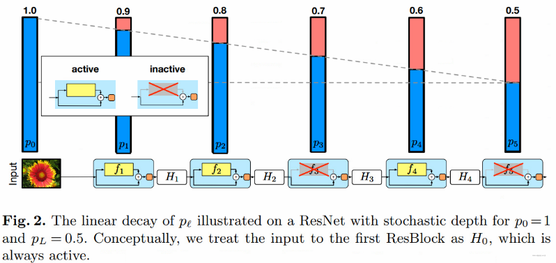
Of course , In practice , The author will “ Linear attenuation law ” Applied to the survival probability of each layer , Because they think earlier layers will extract low-level features , And these basic features are very important to the later layer , Therefore, these layers should not frequently discard the main branch . As the features extracted in the later layer become more and more abstract , Redundancy may be higher , So go to the back , The probability of discarding the main branch increases , The specific calculation formula is as follows ：
$$p_{\ell }=1-\frac{\ell }{L}\left(1-p_L\right)$$
there $p_l$ Express $l$ Retention probability of main branch in layer training ,$L$ yes block Total number of blocks , $p_L$ We gave it dropout_rate.$l$ Is said $l$ The remnant of the layer .

Experiments show that , It's also training a 110 Layer of ResNet, The performance of training at any depth , Better performance than training at a fixed depth . That means ResNet Some layers in （ route ） May be redundant .

So the advantages of this training method ：

1. The results solve the time problem of in-depth network training
2. Greatly reduce training time , And significantly improve the accuracy of the network
3. Can make the network deeper

Of course , The principle here is not very difficult , The following is mainly to see how to implement it from the code level .

Here EfficientNet The code in the network is explained , Others are similar ：

# kernel_size, in_channel, out_channel, exp_ratio, strides, use_SE, drop_connect_rate, repeats
default_cnf = [[3, 32, 16, 1, 1, True, drop_connect_rate, 1],
                [3, 16, 24, 6, 2, True, drop_connect_rate, 2],
                 [5, 24, 40, 6, 2, True, drop_connect_rate, 2],
                 [3, 40, 80, 6, 2, True, drop_connect_rate, 3],
                 [5, 80, 112, 6, 1, True, drop_connect_rate, 3],
                 [5, 112, 192, 6, 2, True, drop_connect_rate, 4],
                 [3, 192, 320, 6, 1, True, drop_connect_rate, 1]]

Here is a list of each stage Configuration of , Don't worry about this , Look at this EfficientNet The network structure of .

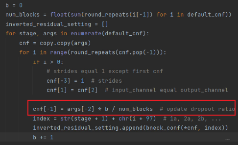
Here is the code to modify the configuration , That is, it will traverse each of the above stage, Then the residual block is established according to the number of repetitions , The residual block here is the inverse residual module , The structure in the figure at the beginning . It's mainly the sentence framed , Namely “ Linear attenuation law ” The formula for , there cnf[-1] Represents the of the current residual block dropout_rate, and args[-2] It's our designated dropout_rate, $b$ At present $l$ layer , num_blocks That's all blocks Count , It corresponds to the above formula one by one .

We'll find out , When building a network , Each residual block specifies a dropout_rate, So in each residual block , We built dropout The layers are as follows , I'll just take it here EfficientNetV1 Look at , Focus on self.dropout that will do , The above ones are the expansion convolution on the main branch ,dw Convolution and dimensionality reduction convolution , Not the point of this article ：

class InvertedResidualEfficientNetV1(nn.Module):
    def __init__(self,
                 cnf: InvertedResidualConfigEfficientNet,
                 norm_layer: Callable[..., nn.Module]):
        super(InvertedResidualEfficientNetV1, self).__init__()
        self.use_res_connect = (cnf.stride == 1 and cnf.input_c == cnf.out_c)
        layers = OrderedDict()
        activation_layer = nn.SiLU  # alias Swish

        # expand
        if cnf.expanded_c != cnf.input_c:
            layers.update({
    "expand_conv": ConvBNActivation(cnf.input_c,
                                                           cnf.expanded_c,
                                                           kernel_size=1,
                                                           norm_layer=norm_layer,
                                                           activation_layer=activation_layer)})

        # depthwise
        layers.update({
    "dwconv": ConvBNActivation(cnf.expanded_c,
                                                  cnf.expanded_c,
                                                  kernel_size=cnf.kernel,
                                                  stride=cnf.stride,
                                                  groups=cnf.expanded_c,
                                                  norm_layer=norm_layer,
                                                  activation_layer=activation_layer)})

        if cnf.use_se:
            layers.update({
    "se": SqueezeExcitationV2(cnf.input_c,
                                                   cnf.expanded_c)})

        # project
        layers.update({
    "project_conv": ConvBNActivation(cnf.expanded_c,
                                                        cnf.out_c,
                                                        kernel_size=1,
                                                        norm_layer=norm_layer,
                                                        activation_layer=nn.Identity)})

        self.block = nn.Sequential(layers)
        self.out_channels = cnf.out_c
        self.is_strided = cnf.stride > 1

        #  Only in use shortcut Only use when connecting dropout layer 
        if self.use_res_connect and cnf.drop_rate > 0:
            self.dropout = DropPath(cnf.drop_rate)
        else:
            self.dropout = nn.Identity()

    def forward(self, x: Tensor) -> Tensor:
        result = self.block(x)
        result = self.dropout(result)
        if self.use_res_connect:
            result += x

The code details here are needless to say , In fact, it is the residual network structure at the beginning , We mainly look at when to use Dropout, Only use the long jump connection , And the current dropout_rate Greater than 0 When , our Dropout The floor will go one DropPath, Otherwise, it is not a residual structure , Or not dropout_rate, Then let's wait and see , therefore DropoutPath For residual structure only .

that DropPath How to achieve it ？

class DropPath(nn.Module):
    def __init__(self, drop_prob=None):
        super(DropPath, self).__init__()
        self.drop_prob = drop_prob

    def forward(self, x):
        return drop_path(x, self.drop_prob, self.training)

Here is a DropPath layer , The core implementation here is drop_path function , In this , The realization is based on the given dropout_rate Probabilistic random deactivation of the main branch . So let's focus on the implementation logic of this ：

def drop_path(x, drop_prob: float = 0, training: bool = False):
    if drop_prob == 0. or not training:
        return x
    keep_prob = 1 - drop_prob

    # ndim Is the number of dimensions  x.shape[0]  It's the number of samples , shape: (x.shape[0], 1, 1, 1)  Dimensions can be used + Splicing 
    shape = (x.shape[0], ) + (1, ) * (x.ndim - 1)

    #  Generate a random number for each sample  torch.rand[0, 1), keep_prob (0, 1],  The sum of the two is [0, 2)  The shape is (x.shape[0], 1, 1, 1)
    random_tensor = keep_prob + torch.rand(shape, dtype=x.dtype, device=x.device)  # torch.rand  Random number extracted from uniform distribution ([0,1))

    #  Round down , namely random_tensor Not 0 namely 1  shape (x.shape[0], 1, 1, 1)
    random_tensor.floor_()    #  Round down 

	#  Here, the random deactivation of the main branch ,  Divide keep_prob To keep the scale of training and testing consistent , Ordinary dropout Ideas 
    output = x.div(keep_prob) * random_tensor
    return output

Here to find out , I annotate every line of code . In fact, the logic is very simple , For one of us batch The sample inside , such as $n$ individual , Then input x The shape of $(n,channe{l}_{size},h,w)$, We'll start with each sample , Will generate a [0,2) Random number between , Then round down , You get non 0 namely 1 Of random_tensor, This is actually our $b_l$, Each sample corresponds to one , So when training each sample , Will see if the main branch is activated . Then whether to activate , That's what the last line of code does , Here divided by keep_prob It is to ensure that the scale range of training set and test set is consistent , And ordinary dropout equally .

such , And that's what happened dropout Technology randomly discards some residual layers .

The reason for this is that , I think this technology is very practical in network training , And it's a general technology , Many models with residual networks can be used , such as resnet, densenet, efficientnet wait , It can speed up the training , It can also increase the network accuracy , very powerful Things that are .

Reference resources ：

• Of deep learning model ——Stochastic depth（ Random depth ）