Machine learning (VI) -- Bayesian classifier

Bayesian classifier is the general name of a class of classification algorithms , Are based on Bayesian theorem

One 、 Preliminary knowledge — Bayesian decision theory

1. The formula

\qquad Bayesian decision theory is the basic method of implementing decision under the framework of probability . For classification tasks , In the ideal case where all relevant probabilities are known , Bayesian decision theory considers how to select the optimal category marker based on probability and misjudgment loss .

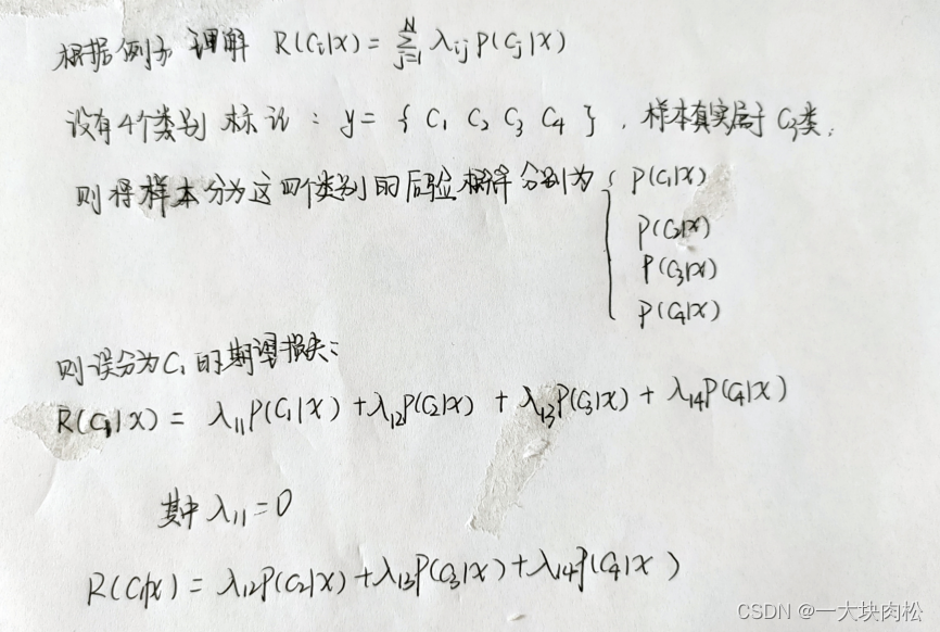
\qquad Suppose there is N Output categories , Expressed as $y$={ $c_1,c_2,c_3.....c_N$}
\qquad ${\lambda }_{ij}$ It means that a real belongs to $c_j$ The samples were misclassified as $c_i$ Loss incurred .
\qquad Then the sample $x$ Classified as $c_i$ The expected loss incurred , In the sample $x$ Upper “ Conditional risk ” by ：

The above formula can be understood as ：

To achieve the correct classification , You need to minimize the expected loss , The above is the expected loss of a single sample , Then the overall loss expectation is ：

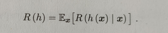
\qquad According to the above formula, we can know , If conditional risk is minimized for each sample , Then the overall risk $R(h)$, It will also be minimized . This produces Bayesian criteria ： To minimize the overall risk , Just select the one on each sample that makes the conditional risk $R(c|x)$ The smallest category mark .

$h^{\ast }$ It's called Bayesian optimal classifier .

2. Minimize classification error rate

Miscalculation of loss ${\lambda }_{ij}$, Set to 0/1 Loss function ：

At this point, conditional risk ：

The origin of the above formula ：

Therefore, the Bayesian optimal classifier to minimize the classification error rate is ：

For each sample $x$, Selection can make a posteriori probability $P(c|x)$ Maximum category tag

3. Posterior probability

\qquad From the above explanation , It is required to minimize the risk of decision-making , First, we need to obtain a posterior probability $P(c|x).$
\qquad From this perspective , The task of machine learning is to estimate the posterior probability as accurately as possible based on the limited training sample set $P(c|x)$, Depending on the generation strategy , It is divided into two models ：

Discriminant model
Generative model
The so-called discriminant model , Direct modeling a posteriori probability $P(c|x).$
The so-called generative model ,: For joint probability distribution $P(c,x)$ modeling , Then we get the posterior probability $P(c|x).$

Generative model ：

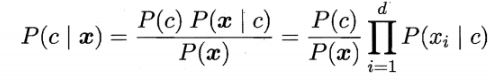
Based on Bayesian theorem, it can be written as ：

among ：$P(c|x)：afterExaminationGeneralrate$
$P(c)：FirstExaminationGeneralrate$
$P(x|c)：likehoweverGeneralrate$

Two 、 Maximum likelihood estimation

According to Bayes theorem ：

Find the maximum a posteriori probability $P(c|x)$ To find the maximum likelihood $P(x|c)$.

\qquad Let the training set be $D$
\qquad The first $c$ The label of the class is ${\theta }_c$
\qquad Ji Youdi c The collection of tags of class is $D_c$（ Personal understanding $D_c：$ It refers to which features in the set can be combined to get ${\theta }_c$ Class sample ）
\qquad Suppose these samples are independent and identically distributed , The parameter ${\theta }_c$ For datasets $D_c$ The likelihood of ：

The above formula is the continuous multiplication operation , Easy to cause underflow , We usually use logarithmic likelihood ：

3、 ... and 、 Naive Bayes classifier

1. Definition

Naive Bayes classifier uses “ Assumption of independence of attribute condition ”： For known categories , Suppose all the attributes are independent of each other .

According to the assumption of attribute conditional independence , Rewritable Bayesian rule ：

That is to maximize ：

Make $D_c$ Represents a training set $D$ pass the civil examinations c Set of class samples , A priori probability can be calculated according to the properties of independent identically distributed $P(c)$：

Make $D_{c,x_i}$ Express $D_c$ In the first place $i$ The value of each attribute is $x_i$ A collection of samples , Then the conditional probability $P(x_i|c)$：

2. Calculation case

Refer to the post

In order to avoid the information carried by other attributes being erased by attribute values that do not appear in the training set , When estimating the probability, we usually have to “ smooth “, Commonly used ” Laprado correction “.

Four 、 Semi naive Bayesian classifier

In a real task , It can not meet the attribute conditions assumed by naive Bayes , That is, it is difficult to establish .
Thus, the semi naive Bayesian classifier is generated

\qquad The basic idea of semi naive Bayesian classifier ： Due consideration should be given to the interdependent information among some attributes , Joint probability calculation is not required , And it doesn't completely ignore the strong attribute dependency .
\qquad ” Independent estimation “（One-Dependent Estimation ,ODE） It is the most commonly used strategy of semi naive Bayesian classifier , That is, it is assumed that each attribute depends on at most one other attribute outside the category , namely

Different approaches , Different dependent classifiers can be generated ：

SPORT
TAN
AODE

5、 ... and 、 Bayesian networks
Bayesian network engraving draws the dependencies between all attributes .
Bayesian networks , It's called “ Faith net ”;
In a real task , Bayesian networks are unknown , We need to find the most appropriate Bayesian network according to the training set .
“ Score search ” Is a common way to solve this problem .

\qquad But reality , It is a problem to find the optimal Bayesian network structure from the training set NP Difficult problem , Difficult to solve quickly .
\qquad There are two common strategies that can solve the approximate solution in a limited time ：
\qquad The first one is ： The law of greed , For example, starting from a certain network structure , Adjust one edge at a time , Until the value of the scoring function no longer decreases ;
\qquad The second kind ： Reduce the search space by imposing constraints on the network structure , For example, the network structure is limited to a tree structure .

5、 ... and 、EM Algorithm

\qquad In the previous discussion , We have always assumed that the values of all attribute variables of the training sample have been observed , The training sample is “ complete ” Of .
\qquad But in practical application, we often encounter “ Incomplete ” Training sample , For example, because the root of watermelon has fallen off , It can't be seen that “ Curl up ” still “ Be stiff ”, Of the training sample “ roots ” Unknown attribute variable value , In this kind of existence ” Not observed “ In the case of variables , Can we still estimate the model parameters ？
For the phenomenon of unknown attribute variables , We can use EM Algorithm
EM The algorithm is a powerful tool to estimate the hidden variables of parameters .

Compared with the previous formula , More $Z$（ Implicit variable set ）

EM The basic idea of algorithm ： If parameter $\theta$ It is known that , Then the optimal hidden variable can be inferred from the training data $Z$ Value （E Step ）; conversely , if $Z$ It is known that , The parameters can be easily adjusted $\theta$ Make maximum likelihood estimation .

6、 ... and 、 Learning materials

zhou ——《 machine learning 》
post 1
post 2