当前位置:网站首页>【图像分类】2017-MobileNetV1 CVPR
【图像分类】2017-MobileNetV1 CVPR
2022-08-10 19:12:00 【說詤榢】
【图像分类】2017-MobileNetV1 CVPR
论文题目:MobileNets: Efficient Convolutional Neural Networks for Mobile Vision Applications
论文链接:论文原地址
论文代码:TensorFlow官方
视频讲解:https://www.bilibili.com/video/BV16b4y117XH
发表时间:2017年4月
引用:Howard A G, Zhu M, Chen B, et al. Mobilenets: Efficient convolutional neural networks for mobile vision applications[J]. arXiv preprint arXiv:1704.04861, 2017.
引用数:14275
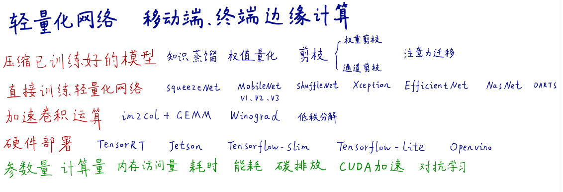
轻量化模型的内容
1. 前期准备
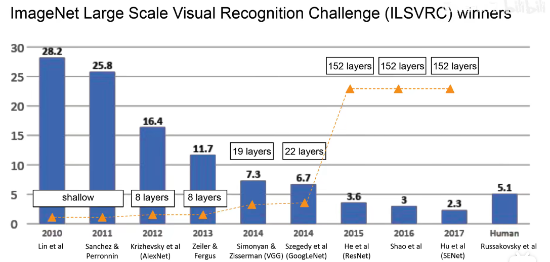
随着计算机视觉的准确率越来越高,到现在已经明显低于人类的失误率。但是这些都是随着网络越来越大,越来越臃肿实现的。精度这个碉堡已经被攻克,所以现在就另找一个方向,就是轻量化,把网络变的简单。
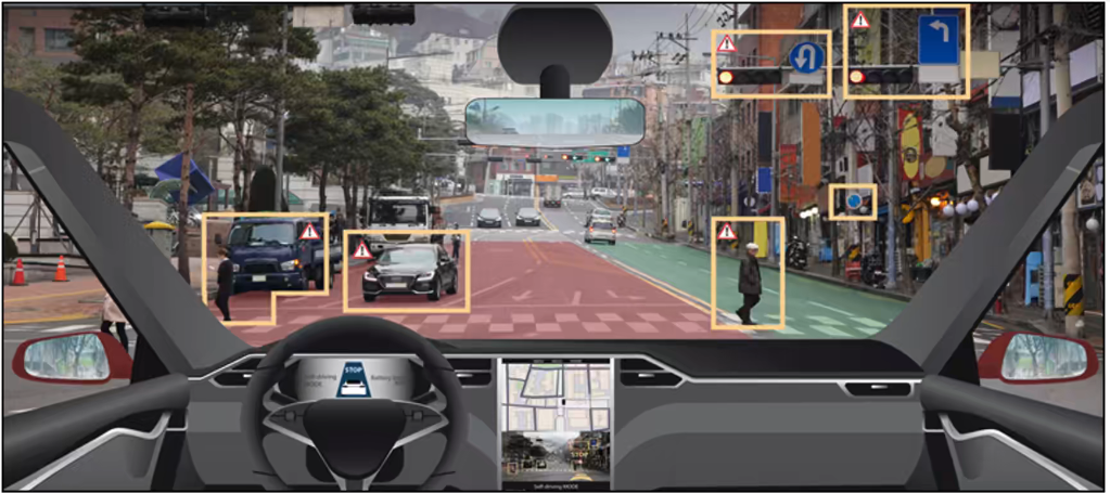
不适合实时边缘计算,比如无人驾驶场景。
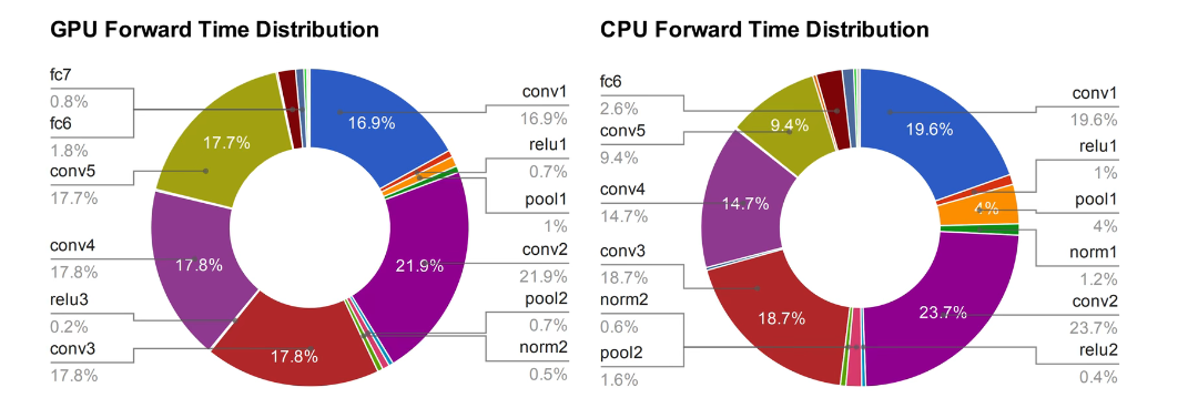
然后,我们对所有操作所花费的时间,做一个时间计算,可以看出卷积操作花费的时间十分的长,所以MobileNet对卷积操作进行了优化。
轻量化的网络的角度和思路
2. 简介
2.1 摘要
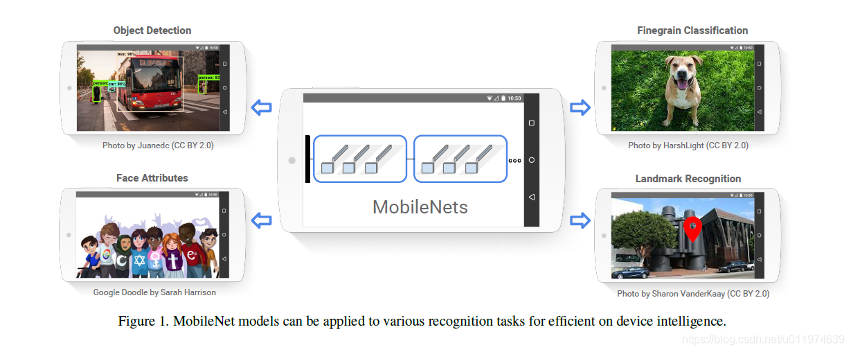
MobileNets是为移动和嵌入式设备提出的高效模型。
MobileNets基于流线型架构(streamlined),使用深度可分离卷积(depthwise separable convolutions,即Xception变体结构)来构建轻量级深度神经网络。
论文介绍了两个简单的全局超参数,可有效的在延迟和准确率之间做折中。这些超参数允许我们依据约束条件选择合适大小的模型。论文测试在多个参数量下做了广泛的实验,并在ImageNet分类任务上与其他先进模型做了对比,显示了强大的性能。论文验证了模型在其他领域(对象检测,人脸识别,大规模地理定位等)使用的有效性。
2.2 简介
深度卷积神经网络将多个计算机视觉任务性能提升到了一个新高度,总体的趋势是为了达到更高的准确性构建了更深更复杂的网络,但是这些网络在尺度和速度上不一定满足移动设备要求。MobileNet描述了一个高效的网络架构,允许通过两个超参数直接构建非常小、低延迟、易满足嵌入式设备要求的模型
2.3 相关工作
现阶段,在建立小型高效的神经网络工作中,通常可分为两类工作:
压缩预训练模型获得小型网络的一个办法是减小、分解或压缩预训练网络,例如量化压缩(product quantization)、哈希(hashing )、剪枝(pruning)、矢量编码( vector quantization)和霍夫曼编码(Huffman coding)等;此外还有各种分解因子(various factorizations )用来加速预训练网络;还有一种训练小型网络的方法叫蒸馏(distillation ),使用大型网络指导小型网络,这是对论文的方法做了一个补充,后续有介绍补充。
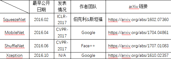
直接训练小型模型。 例如Flattened networks利用完全的因式分解的卷积网络构建模型,显示出完全分解网络的潜力;Factorized Networks引入了类似的分解卷积以及拓扑连接的使用;Xception network显示了如何扩展深度可分离卷积到Inception V3 networks;Squeezenet 使用一个bottleneck用于构建小型网络。
2.4 网络结构和训练
标准卷积和MobileNet中使用的深度分离卷积结构对比如下

注意:如果是需要下采样,则在第一个深度卷积上取步长为2.
MobileNet的具体结构如下(dw表示深度分离卷积):

除了最后的FC层没有非线性激活函数,其他层都有BN和ReLU非线性函数.
我们的模型几乎将所有的密集运算放到 1 × 1 1\times 1 1×1卷积上,这可以使用general matrix multiply (GEMM) functions优化。在MobileNet中有95%的时间花费在 1 × 1 1\times 1 1×1卷积上,这部分也占了75%的参数:

剩余的其他参数几乎都在FC层上了。
在TensorFlow中使用RMSprop对MobileNet做训练,使用类似InceptionV3 的异步梯度下降。与训练大型模型不同的是,我们较少使用正则和数据增强技术,因为小模型不易陷入过拟合;没有使用side heads or label smoothing,我们发现在深度卷积核上放入很少的L2正则或不设置权重衰减的很重要,因为这部分参数很少。
3. V1文章亮点-深度分类卷积
深度分类卷积是对正常的卷积的优化,把一个步骤的卷积操作变成了2步
第一步是DW卷积,第二步是PW卷积
1) DW 卷积
一个卷积核对应一个通道,所以只对宽度和高度上的特征进行了提取,对通道上的信息不做任何树立

2) PW 卷积
pw卷积就是正常的卷积操作,但是卷积核的大小变成了 1 × 1 1\times 1 1×1,作用是跨通道特征提取
3) 深度分类卷积示例
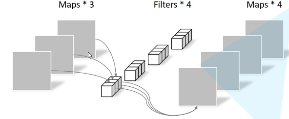
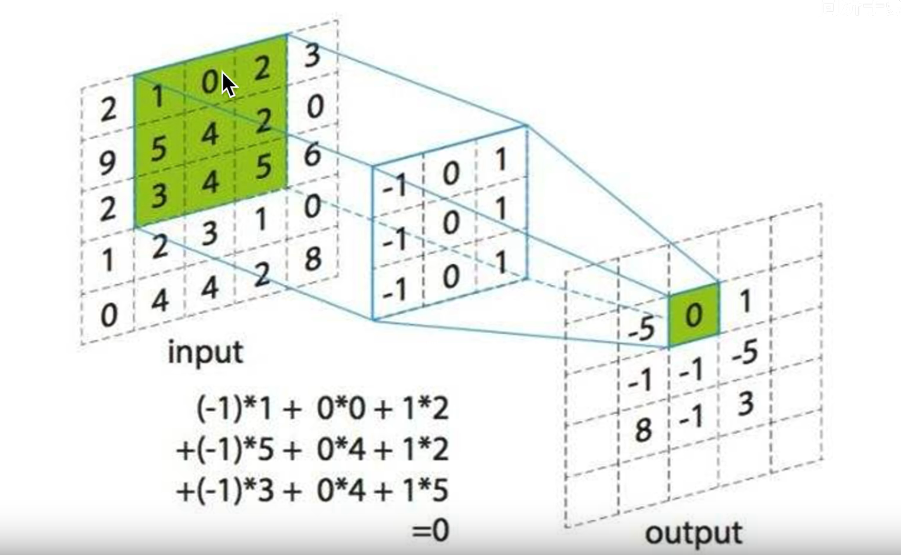
输入图片的大小为 ( 6 , 6 , 3 ) (6,6,3) (6,6,3),原卷积操作是用 ( 4 , 4 , 3 , 5 ) (4,4,3,5) (4,4,3,5)的卷积。 ( 4 × 4 ) (4\times 4) (4×4)是卷积核大小, 3 3 3是卷积通道数, 5 5 5表示卷积核数量, s t r i d e = 1 stride=1 stride=1,没有padding,
输出特征为 6 − 4 1 + 1 = 3 \frac{6-4}{1}+1=3 16−4+1=3,即呼出的特征映射为 ( 3 , 3 , 5 ) (3,3,5) (3,3,5)
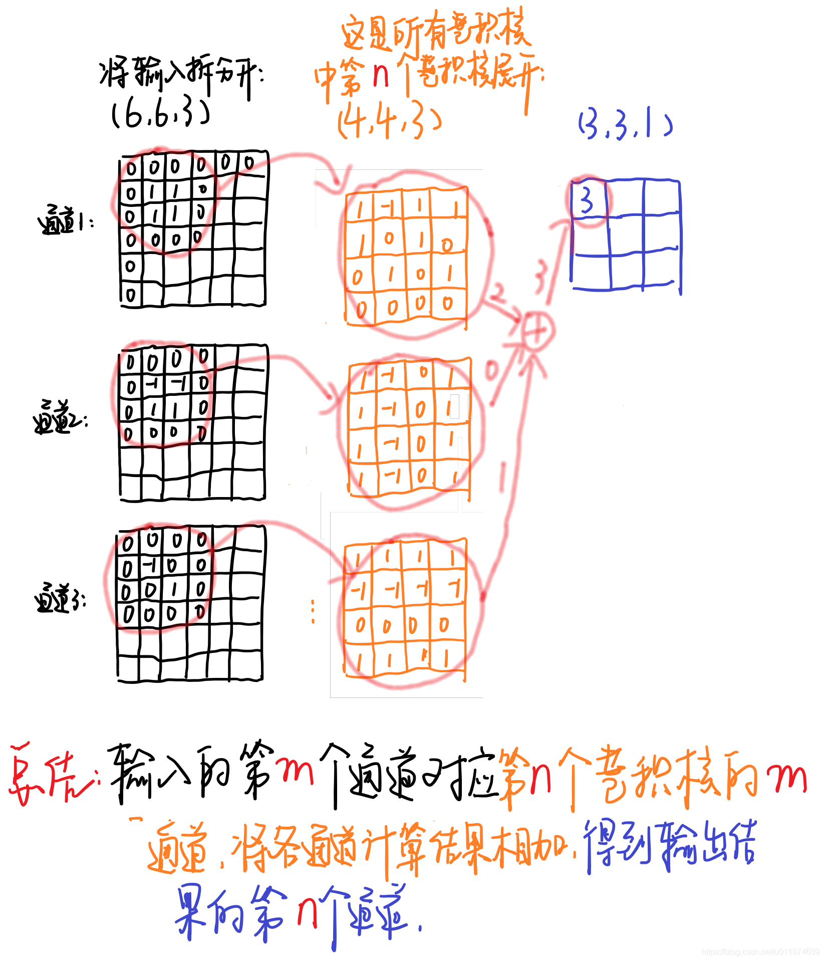
黑色的输入为 ( 6 , 6 , 3 ) (6,6,3) (6,6,3)与第 n n n个卷积核对应,每个通道对应每个卷积核通道卷积得到输出,最终输出为 2 + 0 + 1 = 3 2+0+1=3 2+0+1=3(这是常见的卷积操作,注意这里卷积核要和输入的通道数相同,即图中表示的3个通道~)
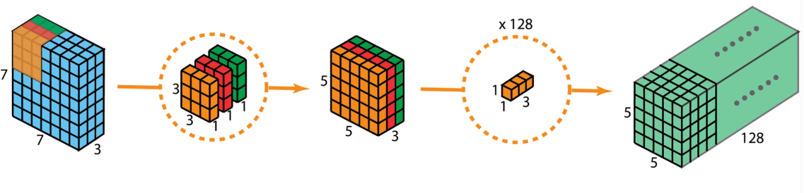
对于深度分离卷积,把标准卷积 ( 4 , 4 , 3 , 5 ) (4,4,3,5) (4,4,3,5)分解为
- 深度卷积部分,大小为 ( 4 , 4 , 1 , 3 ) (4,4,1,3) (4,4,1,3),作用在输入的每个通道上,输出特征映射为 ( 3 , 3 , 3 ) (3,3,3) (3,3,3)
- 逐点卷积部分,大小 ( 1 , 1 , 3 , 5 ) (1,1,3,5) (1,1,3,5),作用在深度卷积的输出特征映射上,得到最终输出为 ( 3 , 3 , 5 ) (3,3,5) (3,3,5)

输入有3个通道,对应着有3个大小为 ( 4 , 4 , 1 ) (4,4,1) (4,4,1)的深度卷积核,卷积结果共有3个大小为 ( 3 , 3 , 1 ) (3,3,1) (3,3,1),我们按顺序将这卷积按通道排列得到输出卷积结果 ( 3 , 3 , 3 ) (3,3,3) (3,3,3)
相比之下计算量减少了:
4 × 4 × 3 × 5 4\times 4\times 3\times 5 4×4×3×5转为了 4 × 4 × 1 × 3 + 1 × 1 × 3 × 5 4\times 4\times 1\times 3+1\times 1\times 3\times 5 4×4×1×3+1×1×3×5即参数量减少了
4 × 4 × 1 × 3 + 1 × 1 × 3 × 5 4 × 4 × 3 × 5 = 21 80 \frac{4\times 4\times 1\times 3+1\times 1\times 3\times 5}{4\times 4\times 3\times 5}=\frac{21}{80} 4×4×3×54×4×1×3+1×1×3×5=8021
MobileNet使用可分离卷积减少了8到9倍的计算量,只损失了一点准确度。
换成数字就是 D k ⋅ D k ⋅ M ⋅ D F ⋅ D f + M ⋅ N ⋅ D F ⋅ D F = D e p t h w i s e + P o i n t w i s e D_k\cdot D_k\cdot M\cdot D_F\cdot D_f+M\cdot N\cdot D_F\cdot D_F=Depthwise+Pointwise Dk⋅Dk⋅M⋅DF⋅Df+M⋅N⋅DF⋅DF=Depthwise+Pointwise
( D k ⋅ D k ) (D_k\cdot D_k) (Dk⋅Dk)就是一次卷积的乘法次数,
( M ⋅ D F ⋅ D F ) (M\cdot D_F\cdot D_F) (M⋅DF⋅DF)输出feature map元素的个数
( N ⋅ D F ⋅ D F ) (N\cdot D_F\cdot D_F) (N⋅DF⋅DF)输出的feature map元素的个数
参数量= D k ⋅ D k ⋅ M + 1 ⋅ 1 ⋅ M ⋅ N D_k\cdot D_k\cdot M+1\cdot1 \cdot M\cdot N Dk⋅Dk⋅M+1⋅1⋅M⋅N
原来参数量= D k ⋅ D k ⋅ M ⋅ N D_k\cdot D_k\cdot M\cdot N Dk⋅Dk⋅M⋅N
换个图解释一下
再换一张图
4. 代码
import time
import torch
import torch.nn as nn
import torch.backends.cudnn as cudnn
import torchvision.models as models
from torch.autograd import Variable


class MobileNet(nn.Module):
    def __init__(self, n_class=1000):
        super(MobileNet, self).__init__()
        self.nclass = n_class

        def conv_bn(inp, oup, stride):
            return nn.Sequential(
                nn.Conv2d(inp, oup, 3, stride, 1, bias=False),
                nn.BatchNorm2d(oup),
                nn.ReLU(inplace=True)
            )

        def conv_dw(inp, oup, stride):
            return nn.Sequential(
                nn.Conv2d(inp, inp, 3, stride, 1, groups=inp, bias=False),
                nn.BatchNorm2d(inp),
                nn.ReLU(inplace=True),

                nn.Conv2d(inp, oup, 1, 1, 0, bias=False),
                nn.BatchNorm2d(oup),
                nn.ReLU(inplace=True),
            )

        self.model = nn.Sequential(
            conv_bn(3, 32, 2),
            conv_dw(32, 64, 1),
            conv_dw(64, 128, 2),
            conv_dw(128, 128, 1),
            conv_dw(128, 256, 2),
            conv_dw(256, 256, 1),
            conv_dw(256, 512, 2),
            conv_dw(512, 512, 1),
            conv_dw(512, 512, 1),
            conv_dw(512, 512, 1),
            conv_dw(512, 512, 1),
            conv_dw(512, 512, 1),
            conv_dw(512, 1024, 2),
            conv_dw(1024, 1024, 1),
            nn.AvgPool2d(7),
        )
        self.fc = nn.Linear(1024, self.nclass)

    def forward(self, x):
        x = self.model(x)
        x = x.view(-1, 1024)
        x = self.fc(x)
        return x


def speed(model, name):
    t0 = time.time()
    input = torch.rand(1, 3, 224, 224).cuda()  # input = torch.rand(1,3,224,224).cuda()
    input = Variable(input, volatile=True)
    t1 = time.time()

    model(input)

    t2 = time.time()
    for i in range(10):
        model(input)
    t3 = time.time()

    torch.save(model.state_dict(), "test_%s.pth" % name)
    print('%10s : %f' % (name, t3 - t2))


if __name__ == '__main__':
    # cudnn.benchmark = True # This will make network slow ??
    resnet18 = models.resnet18(num_classes=2).cuda()
    alexnet = models.alexnet(num_classes=2).cuda()
    vgg16 = models.vgg16(num_classes=2).cuda()
    squeezenet = models.squeezenet1_0(num_classes=2).cuda()
    mobilenet = MobileNet().cuda()

    speed(resnet18, 'resnet18')
    speed(alexnet, 'alexnet')
    speed(vgg16, 'vgg16')
    speed(squeezenet, 'squeezenet')
    speed(mobilenet, 'mobilenet')
参考资料
边栏推荐
- 转铁蛋白(Tf)修饰去氢骆驼蓬碱磁纳米脂质体/香豆素-6脂质体/多柔比星脂质体
- 【greenDao】Cannot access ‘org.greenrobot.greendao.AbstractDaoSession‘ which is a supertype of
- Random函数用法
- idea汉化教程[通俗易懂]
- 线性结构----链表
- Solution for thread not gc-safe when Rider debugs ASP.NET Core
- 多线程与高并发(五)—— 源码解析 ReentrantLock
- Pt/CeO2 monatomic nanoparticles enzyme | H - rGO - Pt @ Pd NPs enzyme | carbon nanotube load platinum nanoparticles peptide modified nano enzyme | leukemia antagonism FeOPtPEG composite nano enzyme
- 今日份bug,点击win10任务栏视窗动态壁纸消失的bug,暂未发现解决方法。
- Apple Font Lookup
猜你喜欢
测试/开发程序员值这么多钱么?“我“不会愿赌服输......
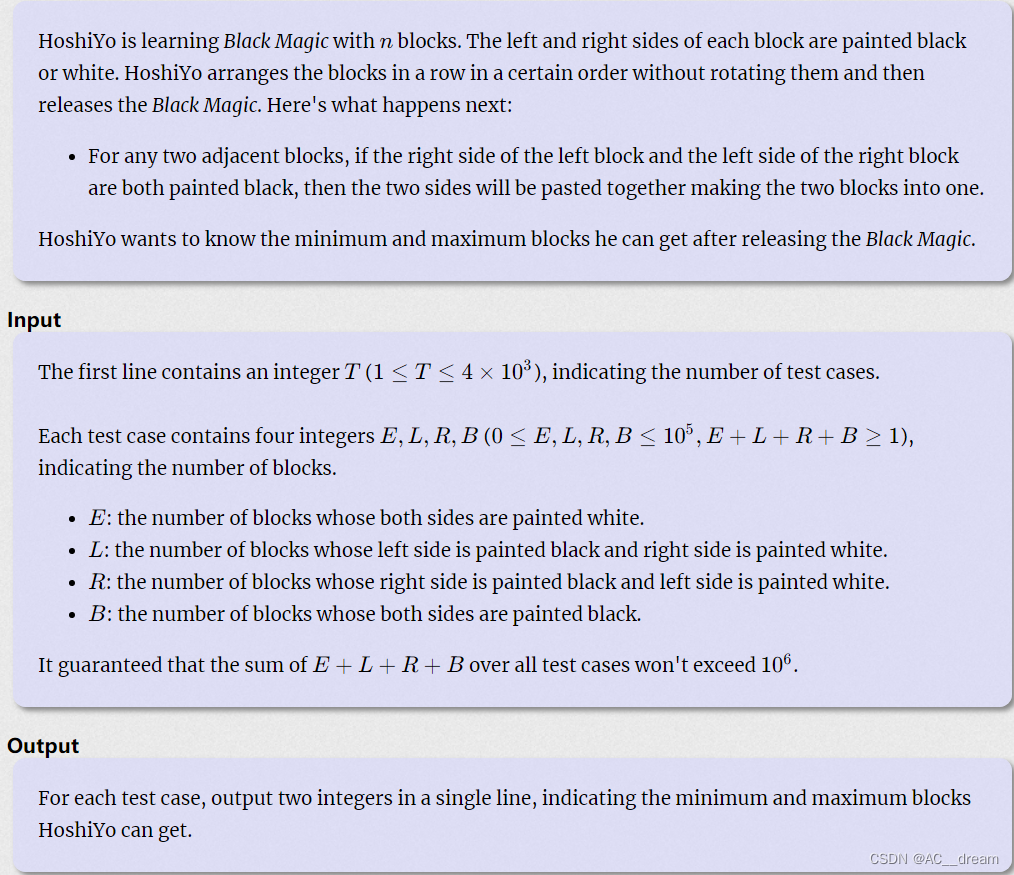
2022 Hangdian Multi-School Seven Black Magic (Sign-in)
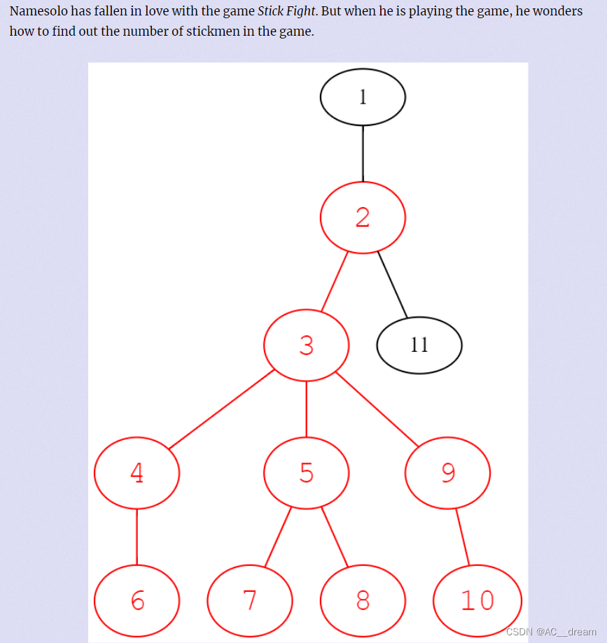
Hangdian Multi-School Seven 1003-Counting Stickmen (Combination Mathematics)
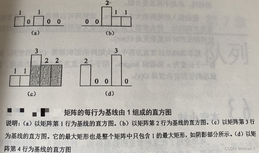
leetcode 85.最大矩形 单调栈应用
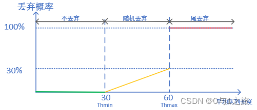
QoS Quality of Service Eight Congestion Avoidance
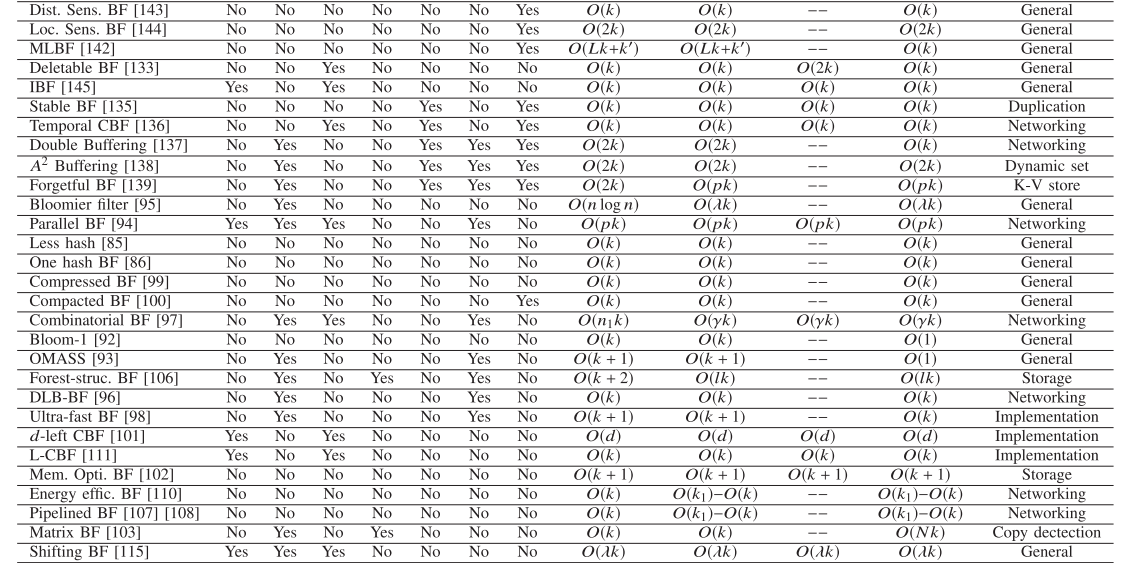
Optimizing Bloom Filter: Challenges, Solutions, and Comparisons论文总结
你不知道的浏览器页面渲染机制
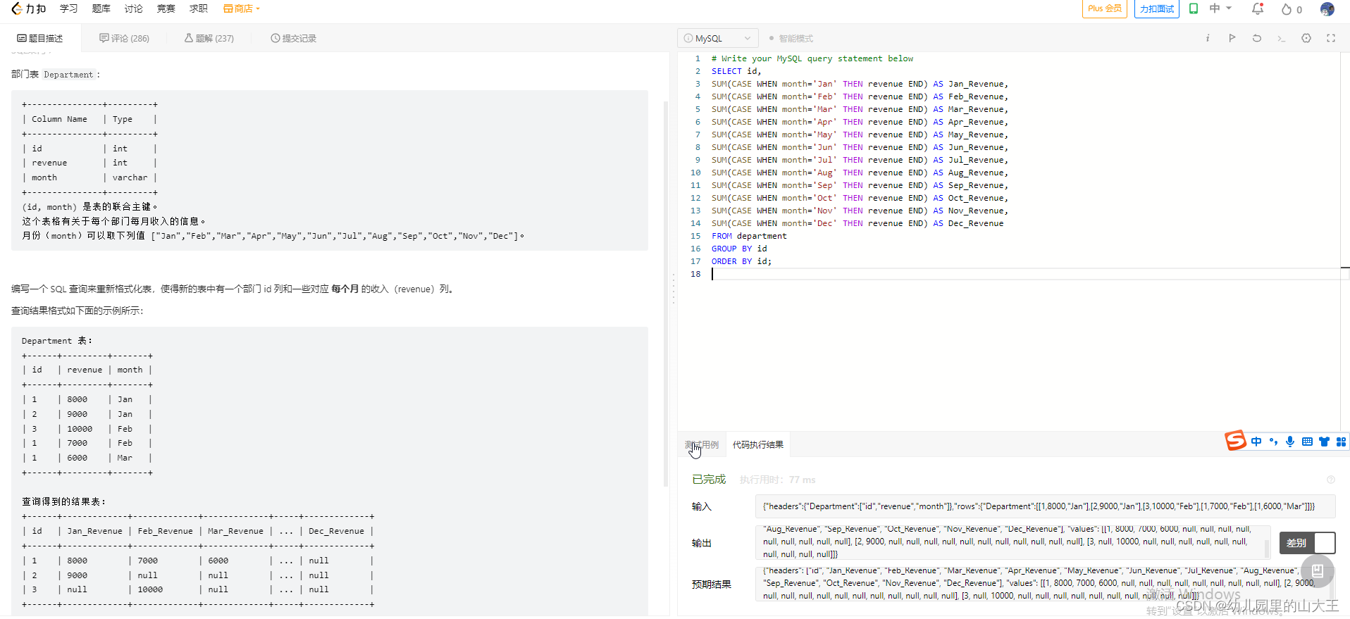
mysql踩坑----case when then用法

网站架构探测&chrome插件用于信息收集
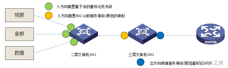
QoS服务质量七交换机拥塞管理
随机推荐
(十)图像数据的序列与反序列化
QoS服务质量七交换机拥塞管理
argparse——命令行参数解析
Site Architecture Detection & Chrome Plugin for Information Gathering
【毕业设计】基于STM32的天气预报盒子 - 嵌入式 单片机 物联网
leetcode 547.省份数量 并查集
(十二) findContours函数的hierarchy详解
网站架构探测&chrome插件用于信息收集
mysql踩坑----case when then用法
mysql----group by、where以及聚合函数需要注意事项
这7个自动化办公模版 教你玩转表格数据自动化
【SemiDrive源码分析】【MailBox核间通信】52 - DCF Notify 实现原理分析 及 代码实战
whois信息收集&企业备案信息
史上最全GIS相关软件(CAD、FME、Arcgis、ArcgisPro)
转铁蛋白(TF)修饰紫杉醇(PTX)脂质体(TF-PTX-LP)|转铁蛋白(Tf)修饰姜黄素脂质体
laya打包发布apk
Multifunctional Nanozyme Ag/PANI | Flexible Substrate Nano ZnO Enzyme | Rhodium Sheet Nanozyme | Ag-Rh Alloy Nanoparticle Nanozyme | Iridium Ruthenium Alloy/Iridium Oxide Biomimetic Nanozyme
When selecting a data destination when creating an offline synchronization node - an error is reported in the table, the database type is adb pg, what should I do?
铱钌合金/氧化铱仿生纳米酶|钯纳米酶|GMP-Pd纳米酶|金钯复合纳米酶|三元金属Pd-M-Ir纳米酶|中空金铂合金纳米笼核-多空二氧化硅壳纳米酶
[教你做小游戏] 只用几行原生JS,写一个函数,播放音效、播放BGM、切换BGM