当前位置:网站首页>Machine learning - logistic regression
Machine learning - logistic regression
2022-04-23 15:18:00 【Please call me Lei Feng】
One 、 Binomial logistic regression
1. Binomial logistic regression is a function , Final output between 0 To 1 Between the value of the , To solve problems similar to “ Success or failure ”,“ Yes or no " such ” No matter whether or not " The problem of .
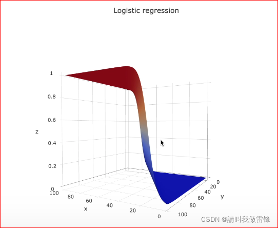
2. Logistic regression is a model that maps linear regression model to probability , That is, the output of real number space [-∞,+∞] Mapping to (0,1), So as to obtain the probability .( Personal understanding : The meaning of regression —— The process of making cognition close to truth with observation , Back to the original .)
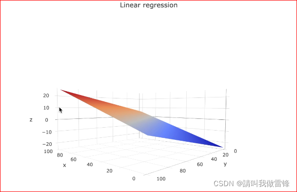
3. We can intuitively understand this mapping through drawing , We first define a binary linear regression model :
y ^ = θ 1 x 1 + θ 2 x 2 + b i a s , Its in y ^ ∈ ( − ∞ , + ∞ ) \hat{y}=\theta_1x_1+\theta_2x_2+bias, among \hat{y}∈(-∞,+∞) y^=θ1x1+θ2x2+bias, Its in y^∈(−∞,+∞)
Linear regression chart :
Logistic regression diagram :
Two 、probability and odds The definition of
1.probability refer to Number of occurrences / The total number of times , Take the coin toss, for example :
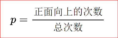
p The value range of is [0,+∞)
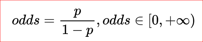
2.odds Is a ratio , It refers to the possibility of an event ( probability ) And the possibility of not happening ( probability ) The ratio of the . namely Number of occurrences / The number of times it didn't happen , Take the coin toss, for example :
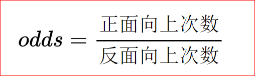
odds The value range of is [0,+∞)
3. Review the Bernoulli distribution : If X Is a random variable in Bernoulli distribution ,X The values for {0,1}, Not 0 namely 1, Such as the front and back of a coin flip :
be :P(X=1)=p,P(X=0)=1-p
Plug in odds:
3、 ... and 、logit Functions and sigmoid Functions and their properties :
1.Odds The logarithm of is called Logit, Also writing log-it.
2. We are right. odds take log, Expand odds The value range of is from the space of real numbers [-∞,+∞], This is it. logit function :
l o g i t ( p ) = l o g e ( o d d s ) = l o g e ( p 1 − p ) , p ∈ ( 0 , 1 ) , l o g i t ( p ) ∈ ( − ∞ , + ∞ ) logit(p)=log_e(odds)=log_e(\frac{p}{1-p}),p∈(0,1),logit(p)∈(-∞,+∞) logit(p)=loge(odds)=loge(1−pp),p∈(0,1),logit(p)∈(−∞,+∞)
3. We can use linear regression model to express logit§, Because linear regression model and logit The output function has the same range of values :
for example : l o g i t ( p ) = θ 1 x 1 + θ 2 x 2 + b i a s logit(p)=\theta_1x_1+\theta_2x_2+bias logit(p)=θ1x1+θ2x2+bias
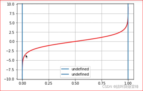
Here are logit§ Function image of , Be careful p∈(0,1), When p=0 perhaps p=1 when ,logit Belongs to undefined .
from l o g i t ( p ) = θ 1 x 1 + θ 2 x 2 + b i a s logit(p)=\theta_1x_1+\theta_2x_2+bias logit(p)=θ1x1+θ2x2+bias
have to
l o g ( p 1 − p ) = θ 1 x 1 + θ 2 x 2 + b i a s log(\frac{p}{1-p} )=\theta_1x_1+\theta_2x_2+bias log(1−pp)=θ1x1+θ2x2+bias
notes : Some people may have misunderstandings , Don't understand how to convert ,logit§ Represents the and parameter p Related logarithmic function , ad locum
logit( p )=log(p/(1-p)).
set up z = θ 1 x 1 + θ 2 x 2 + b i a s z=\theta_1x_1+\theta_2x_2+bias z=θ1x1+θ2x2+bias
have to l o g ( p 1 − p ) = z log(\frac{p}{1-p} )=z log(1−pp)=z
Take... On both sides of the equation e The exponential function of the enemy :
p 1 − p = e z \frac{p}{1-p}=e^{z} 1−pp=ez
p = e z ( 1 − p ) = e z − e z p p=e^{z}(1-p)=e^{z}-e^{z}p p=ez(1−p)=ez−ezp
p ( 1 + e z ) = e z p(1+e^z)=e^z p(1+ez)=ez
p = e z ( 1 + e z ) p=\frac{e^z}{(1+e^z)} p=(1+ez)ez
Both numerator and denominator are divided by e z e^z ez, have to
p = 1 ( 1 + e − z ) , p ∈ ( 0 , 1 ) p=\frac{1}{(1+e^{-z})} ,p∈(0,1) p=(1+e−z)1,p∈(0,1)
After the above derivation , We have come to sigmoid function , Finally, the value of the real number space output by the linear regression model is mapped into probability .
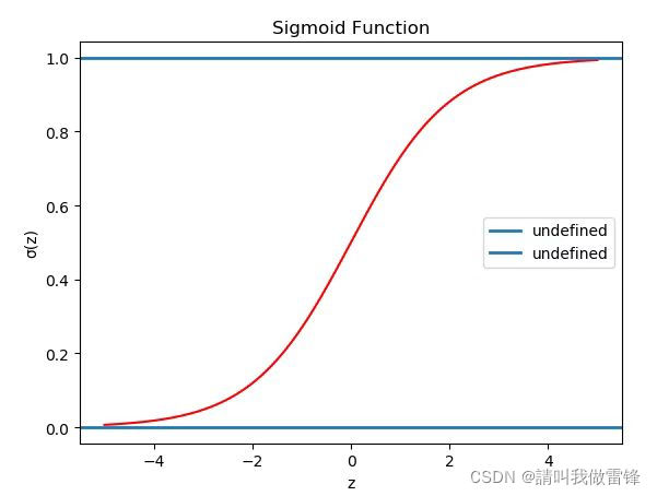
s i g m o i d ( z ) = 1 1 + e − z , p ∈ ( 0 , 1 ) sigmoid(z)=\frac{1}{1+e^{-z}} ,p∈(0,1) sigmoid(z)=1+e−z1,p∈(0,1)
Here is sigmoid Function image of , Be careful sigmoid(z) Value range of
Four 、 Maximum likelihood estimation
1. The assumption function is introduced h θ ( X ) h_\theta(X) hθ(X), set up θ T X \theta^TX θTX It is a linear regression model :
θ T X \theta^TX θTX in , θ T \theta^T θT and X All vectors are columns , for example :
θ T = [ b i a s θ 1 θ 2 ] \theta^T=\begin{bmatrix} bias & \theta_1 &\theta_2 \end{bmatrix} θT=[biasθ1θ2]
X = [ 1 x 1 x 2 ] X=\begin{bmatrix} 1 \\ x_1 \\ x_2 \end{bmatrix} X=⎣⎡1x1x2⎦⎤
Find the dot product of the matrix , obtain :
θ T X = b i a s ∗ 1 + θ 1 ∗ x 1 + θ 2 ∗ x 2 = θ 1 x 1 + θ 2 ∗ x 2 + b i a s \theta^TX=bias*1+\theta_1*x_1+\theta_2*x_2=\theta_1x_1+\theta_2*x_2+bias θTX=bias∗1+θ1∗x1+θ2∗x2=θ1x1+θ2∗x2+bias
set up θ T X = z \theta^TX=z θTX=z, Then there is a hypothetical function :
h θ ( X ) = 1 1 + e − z = P ( Y = 1 ∣ X ; θ ) h_\theta (X)=\frac{1}{1+e^{-z}} =P(Y=1|X;\theta ) hθ(X)=1+e−z1=P(Y=1∣X;θ)
The above expression is under the condition X and θ \theta θ Next Y=1 Probability ;
P ( Y = 1 ∣ X ; θ ) = 1 − h θ ( X ) P(Y=1|X;\theta )=1-h_\theta(X) P(Y=1∣X;θ)=1−hθ(X)
The above expression is under the condition X and θ \theta θ Next Y=1=0 Probability .
2. Review the Bernoulli distribution
f ( k ; p ) { p , i f k = 1 q = 1 − p , i f k = 0 f(k;p)\left\{\begin{matrix} p, &if&k=1 \\ q=1-p, &if&k=0 \end{matrix}\right. f(k;p){
p,q=1−p,ififk=1k=0
perhaps f ( k ; p ) = p k ( 1 − p ) 1 − k f(k;p)=p^k(1-p)^{1-k} f(k;p)=pk(1−p)1−k,for k∈{0,1}. Be careful f(k;p) It means k by 0 or 1 Probability , That is to say P(k)
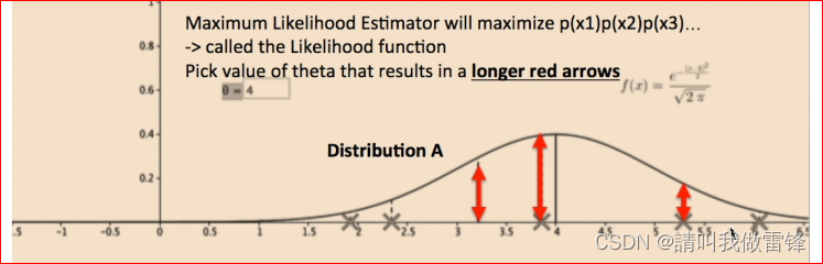
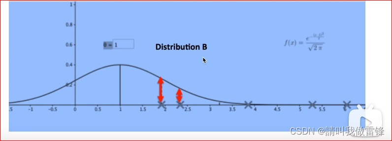
3. The purpose of maximum likelihood estimation is to find a probability distribution that best matches the data .
For example XX Refers to data points , The product of the lengths of all the red arrows in the figure is the output of the likelihood function , obviously , The distribution likelihood function of the upper graph is larger than that of the lower graph , So the distribution of the upper graph is more consistent with the data , Maximum likelihood estimation is to find a distribution that best matches the current data .
4. Define the likelihood function
L ( θ ∣ x ) = P ( Y ∣ X ; θ ) = ∏ i m P ( y i ∣ x i ; θ ) = ∏ i m h θ ( x i ) y i ( 1 − h θ ( x i ) ) ( 1 − y i ) L(\theta|x)=P(Y|X;\theta )=\prod_{i}^{m} P(y_i|x_i;\theta )=\prod_{i}^{m} h_\theta(x_i)^{y_i}(1-h_\theta(x_i))^{(1-{y_i})} L(θ∣x)=P(Y∣X;θ)=i∏mP(yi∣xi;θ)=i∏mhθ(xi)yi(1−hθ(xi))(1−yi),
among i For each data sample , share m Data samples , The purpose of maximum likelihood estimation is to make the above formula “ From output value ” As big as possible ; Top-down extraction log, To facilitate calculation , because log You can convert a product into an addition , And it doesn't affect our optimization goal :
L ( θ ∣ x ) = l o g ( P ( Y ∣ X ; θ ) ) = ∑ i = 1 m y i l o g ( h θ ( x i ) ) + ( 1 − y i ) l o g ( 1 − h θ ( x i ) ) L(\theta|x)=log(P(Y|X;\theta ))=\sum_{i=1}^{m} y_ilog(h_\theta (x_i))+(1-y_i)log(1-h_\theta (x_i)) L(θ∣x)=log(P(Y∣X;θ))=i=1∑myilog(hθ(xi))+(1−yi)log(1−hθ(xi))
We just need to add a minus sign in front of the formula , Then the maximum can be transformed into the minimum , set up h θ ( X ) = Y ^ h_\theta (X)=\hat{Y} hθ(X)=Y^, Get the loss function J ( θ ) J(\theta) J(θ), We just minimize this function , We can get what we want by deriving θ \theta θ:
J ( θ ) = − ∑ i m Y l o g ( Y ^ ) − ( 1 − Y ) l o g ( 1 − Y ^ ) J(\theta)=-\sum_{i}^{m} Ylog(\hat{Y})-(1-Y)log(1-\hat{Y}) J(θ)=−i∑mYlog(Y^)−(1−Y)log(1−Y^)
版权声明
本文为[Please call me Lei Feng]所创,转载请带上原文链接,感谢
https://yzsam.com/2022/04/202204231508367089.html
边栏推荐
- Modify the default listening IP of firebase emulators
- The win10 taskbar notification area icon is missing
- like和regexp差别
- Thinkphp5 + data large screen display effect
- 【thymeleaf】处理空值和使用安全操作符
- Borui data and F5 jointly build the full data chain DNA of financial technology from code to user
- setcontext getcontext makecontext swapcontext
- G007-HWY-CC-ESTOR-03 华为 Dorado V6 存储仿真器搭建
- Kubernetes详解(十一)——标签与标签选择器
- Detailed explanation of C language knowledge points - data types and variables [2] - integer variables and constants [1]
猜你喜欢
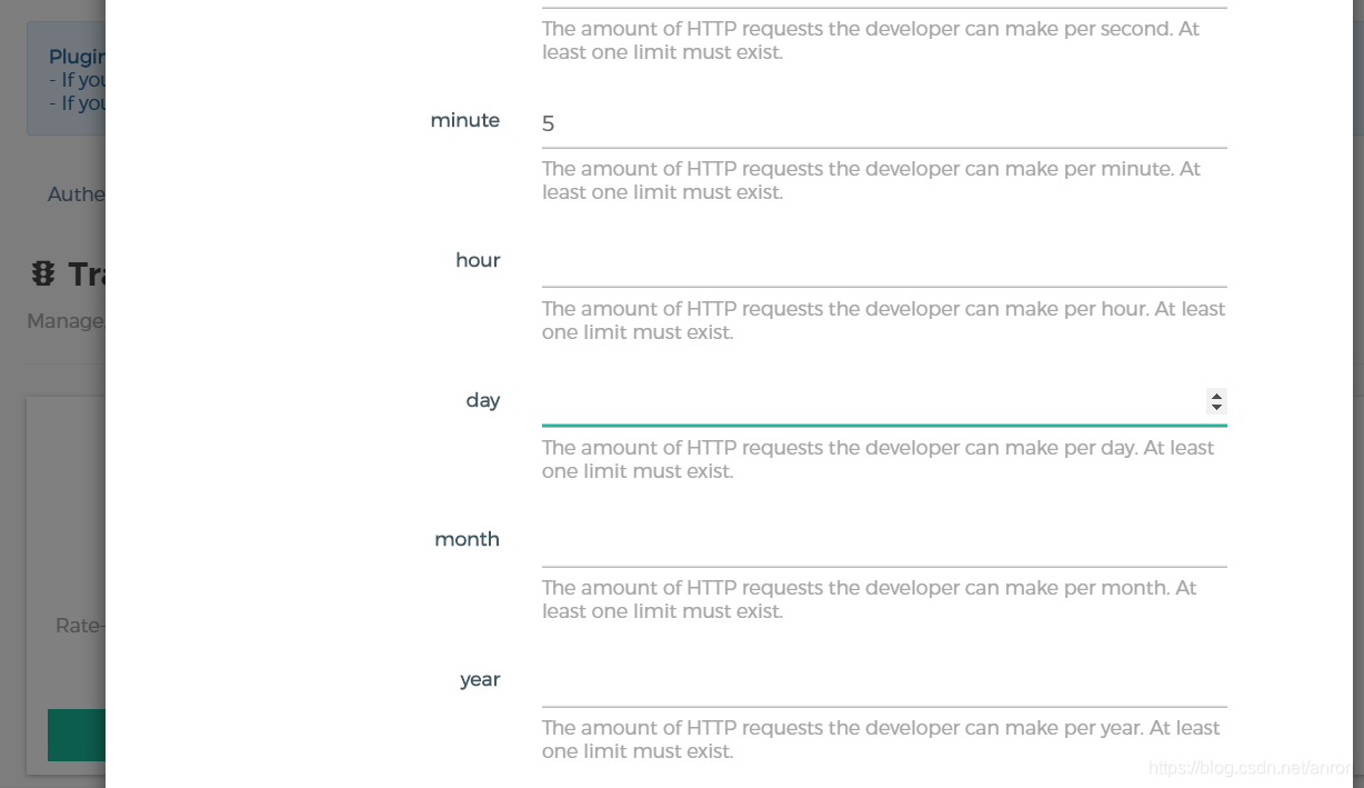
API gateway / API gateway (III) - use of Kong - current limiting rate limiting (redis)
Five data types of redis
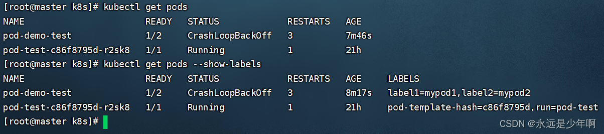
Detailed explanation of kubernetes (XI) -- label and label selector
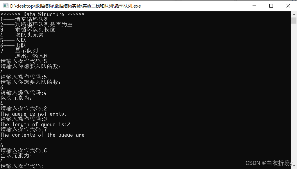
Have you learned the basic operation of circular queue?
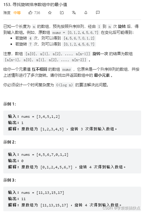
LeetCode153-寻找旋转排序数组中的最小值-数组-二分查找

LeetCode165-比较版本号-双指针-字符串
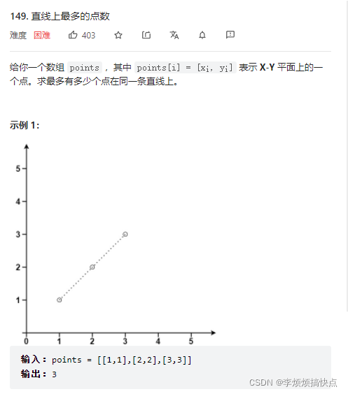
LeetCode149-直线上最多的点数-数学-哈希表

How to design a good API interface?
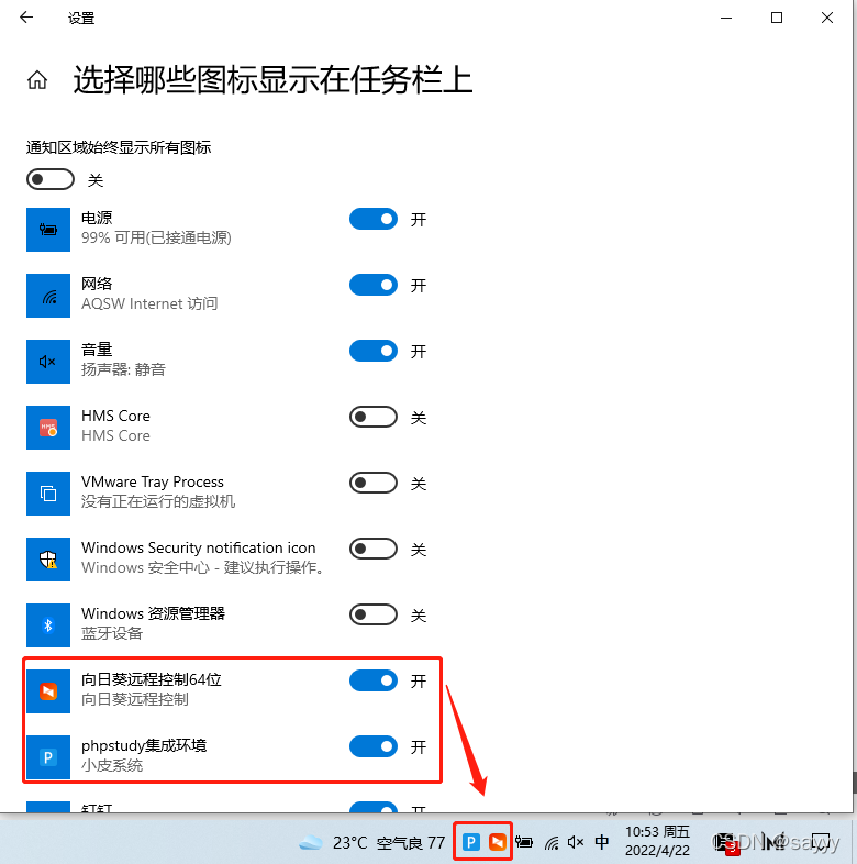
win10 任务栏通知区图标不见了

How to use OCR in 5 minutes
随机推荐
win10 任务栏通知区图标不见了
Differential privacy (background)
HJ31 单词倒排
Lotus DB design and Implementation - 1 Basic Concepts
Share 20 tips for ES6 that should not be missed
Openfaas practice 4: template operation
TLS / SSL protocol details (30) RSA, DHE, ecdhe and ecdh processes and differences in SSL
牛客网数据库SQL实战详细剖析(26-30)
JS - implémenter la fonction de copie par clic
Practice of unified storage technology of oppo data Lake
免费在upic中设置OneDrive或Google Drive作为图床
Daily question - leetcode396 - rotation function - recursion
Leetcode162 - find peak - dichotomy - array
Detailed explanation of C language knowledge points -- first understanding of C language [1] - vs2022 debugging skills and code practice [1]
分享3个使用工具,在家剪辑5个作品挣了400多
UML learning_ Day2
Comment eolink facilite le télétravail
Elk installation
Adobe Illustrator menu in Chinese and English
如何设计一个良好的API接口?