当前位置:网站首页>Tensorflow 2 basic operation dictionary
Tensorflow 2 basic operation dictionary
2022-04-23 20:18:00 【smile-yan】
Instructions for use
Make clear what you need to check , For example, a function tf.split etc. , Then directly use the search function of the browser to find .
Tensorflow2 Basic operation dictionary
- 1. Installation and related data
- 2. tensor Basics
- 3. tensor Three core operations
- 4. tf Mathematical operation of
- 5. tensor High order operation of
- 6. Data loading
- 7. summary
1. Installation and related data
1.1 install
Environmental statement :
- python3
- pip
Installation command ( With 2.3.0 Version as an example ):
pip install tensorflow -i https://pypi.tuna.tsinghua.edu.cn/simple
View version :
pip show tensorflow
If a mirror is found to be too slow , Consider other Download Image addresses :
- https://mirrors.aliyun.com/pypi/simple/
- https://pypi.douban.com/simple/
1.2 The first program
application tensorflow2 The mathematical calculation in .
import tensorflow as tf

A = tf.constant([[1, 2], [3, 4]])
B = tf.constant([[5, 6], [7, 8]])
C = tf.matmul(A, B)

print(C)
Output content :
tf.Tensor(
[[19 22]
 [43 50]], shape=(2, 2), dtype=int32)
1.3 Second procedure
A simple example of handwritten numeral recognition .
import tensorflow as tf

#  Load data
mnist = tf.keras.datasets.mnist

(x_train, y_train), (x_test, y_test) = mnist.load_data()
x_train, x_test = x_train / 255.0, x_test / 255.0
model = tf.keras.models.Sequential([
  tf.keras.layers.Flatten(input_shape=(28, 28)),
  tf.keras.layers.Dense(128, activation='relu'),
  tf.keras.layers.Dropout(0.2),
  tf.keras.layers.Dense(10, activation='softmax')
])

model.compile(optimizer='adam',
              loss='sparse_categorical_crossentropy',
              metrics=['accuracy'])

model.fit(x_train, y_train, epochs=10)

print(model.evaluate(x_test,  y_test, verbose=2))
Output contents include :
Epoch 1/10
1875/1875 [==============================] - 3s 2ms/step - loss: 0.2942 - accuracy: 0.9140
Epoch 2/10
1875/1875 [==============================] - 3s 2ms/step - loss: 0.1431 - accuracy: 0.9573
Epoch 3/10
1875/1875 [==============================] - 3s 1ms/step - loss: 0.1080 - accuracy: 0.9676
Epoch 4/10
1875/1875 [==============================] - 3s 1ms/step - loss: 0.0900 - accuracy: 0.9721
Epoch 5/10
1875/1875 [==============================] - 3s 1ms/step - loss: 0.0775 - accuracy: 0.9760
Epoch 6/10
1875/1875 [==============================] - 3s 2ms/step - loss: 0.0654 - accuracy: 0.9789
Epoch 7/10
1875/1875 [==============================] - 3s 2ms/step - loss: 0.0579 - accuracy: 0.9814
Epoch 8/10
1875/1875 [==============================] - 3s 2ms/step - loss: 0.0535 - accuracy: 0.9827
Epoch 9/10
1875/1875 [==============================] - 3s 2ms/step - loss: 0.0486 - accuracy: 0.9842
Epoch 10/10
1875/1875 [==============================] - 3s 2ms/step - loss: 0.0451 - accuracy: 0.9850
313/313 - 0s - loss: 0.0702 - accuracy: 0.9796
[0.07019094377756119, 0.9796000123023987]
1.4 Relevant documents
- Official website API file It is the simplest, direct and efficient query address
- Video tutorial Choose... For yourself B Learn from some videos on the website
- Long Shu A book written by Mr. long , Provide PPT And source code , It's worth learning . Remember to give it to Mr. long github Point star .
- Provided by Mr. long Paid video tutorial
*《 Deep learning : be based on Keras Of Pythons
2. tensor Basics
2.1 data type
Data types include
- value type (int, float, double)
- Character type (string)
- Boolean type (bool)
The numerical types are often classified according to the number of dimensions :
- Scalar (Scalar). A single real number , Such as 1.2, 3.4 etc. , dimension (Dimension) The number of 0,shape by [ ].
- vector (Vector). n n n An ordered set of real numbers , Wrap... In square brackets , Such as [1.2],[1.2,3.4] etc. , Dimension
by 1, The length is variable ,shape by [n] - matrix (Matrix). n n n That's ok m m m A finite set of column real numbers . such as [ [1, 2 ], [3,4] ]
- tensor (tensor). Generally, scalar 、 Vectors and matrices are collectively referred to as tensors .( All are tensor The object of )
2.2 See if the variable is tensor
import tensorflow as tf
a = 2
print(tf.is_tensor(a)) # False
b = tf.constant(2)
print(tf.is_tensor(b)) # True
Be careful tf.is_tensor() and isinstance The difference between :
import tensorflow as tf

b = tf.constant(2)
print(tf.is_tensor(b)) # True
print(isinstance(b, tf.Tensor)) # True

b = tf.Variable(b)
print(tf.is_tensor(b)) # True
print(isinstance(b, tf.Tensor)) # False
Although in b Has been transformed into tf.Variable type , But it is still tensor type , but isinstance The function returns False, Therefore, it is recommended to use tf.is_tensor function .
2.3 Convert to tensor
import tensorflow as tf
a = 2
print(tf.is_tensor(a)) # False
a = tf.convert_to_tensor(a)
print(tf.is_tensor(a)) # True
2.4 Convert to tensor And change the data type
import tensorflow as tf

a = 123
a = tf.convert_to_tensor(a, dtype=tf.float32)
print(a.dtype) # <dtype: 'float32'>
2.5 Data type conversion
import tensorflow as tf

a = 123

a = tf.cast(a, dtype=tf.float32)
print(a.dtype)             # <dtype: 'float32'>
print(tf.is_tensor(a))     # True

b = [0,1]
b = tf.cast(b, dtype=tf.bool)
print(b.dtype)             # <dtype: 'bool'>
print(tf.is_tensor(b))     # True
2.6 tf.Variable( Optimizeable parameters )
Use tf.Variable Modify a variable , Represents that this variable is a parameter that can be optimized , In the loop iteration, the value of this parameter will be changed to achieve a better overall effect .
import tensorflow as tf
param = 2.4
param = tf.Variable(param)
print(tf.is_tensor(param))    # True
print(param.dtype)            # <dtype: 'float32'>
2.7 View variable dimensions
import tensorflow as tf
a = tf.constant(1)
print(a.ndim)               # 0
print(a.shape)              # ()

b = tf.constant([1,2,3,4])
print(b.ndim)               # 1
print(b.shape)              # (4,)

c = tf.constant([[1,2],[3,4]])
print(c.ndim)               # 2
print(c.shape)              # (2,2)
2.8 See if variables can be optimized trainable
import tensorflow as tf

a = tf.constant([1,2,3,4])
# print(a.trainable) #  Run this line and report an error  has no attribute 'trainable'

a = tf.Variable(a)
print(a.trainable)        # True
2.9 establish tensor Methods
2.9.1 constant function
import tensorflow as tf
tf.constant([1,2])
2.9.2 from numpy or list Data conversion
import numpy as np
import tensorflow as tf

ary = np.array([1,2,3])
a = tf.convert_to_tensor(ary)
print(a.dtype)                # <dtype: 'int64'>
print(tf.is_tensor(a))        # True
2.9.3 tf.zeros、tf.ones function
import tensorflow as tf

a = tf.zeros([2,3])
print(a.dtype)               # <dtype: 'float32'>
print(tf.is_tensor(a))       # True

b = tf.ones([2,3])
print(b.dtype)               # <dtype: 'float32'>
print(tf.is_tensor(b))       # True
2.9.4 tf.fill function 、tf.range function
import tensorflow as tf

c = tf.fill([1,2,3],110)
print(c.dtype)               # <dtype: 'int32'>
print(tf.is_tensor(c))       # True

d = tf.range(40)
print(c.dtype)               # <dtype: 'int32'>
print(tf.is_tensor(c))       # True
2.9.5 tf.random
import tensorflow as tf

#  Chint distribution
a = tf.random.normal([2,3],mean=1,stddev=1)
print(a.dtype)               # <dtype: 'float32'>
print(tf.is_tensor(a))       # True

#  Uniform distribution
b = tf.random.uniform([2,3],minval=0,maxval=1)
print(b.dtype)               # <dtype: 'float32'>
print(tf.is_tensor(b))       # True

#  Random disruption
c = tf.range(50)
tf.random.shuffle(c)
print(c.dtype)               # <dtype: 'int32'>
print(tf.is_tensor(c))       # True
3. tensor Three core operations
To make it easier to explain , Appointment
- [b, h, w] Express b Zhang High for h, Wide for w Pictures of the .
- [b, h, w, 3] Express b Zhang High for h, Wide for w The color picture of , final [3] Indicates the corresponding RGB value .
- [50,28,28] Express 50 Zhang 28x28 Pictures of the .
- [50,28,28,3] Express 50 Zhang 28x28 The color picture of .
3.1 Index and slice
3.1.1 The most basic indexing method data[1][2]…
import tensorflow as tf

data = tf.random.normal([50,28,28],mean=1,stddev=1)
#  Get the last value of the first pixel of the picture
print(data[0][27][27])
#  Get all pixel values in the first row of the first picture
print(data[0][0])
#  Get the pixel value matrix of the second picture
print(data[1])
3.1.2 Short square brackets data[1,2,3]
import tensorflow as tf

data = tf.random.normal([50,28,28],mean=1,stddev=1)
#  Get the last value of the first pixel of the picture
print(data[0,27,27])
#  Get all pixel values in the first row of the first picture
print(data[0,0])
#  Get the pixel value matrix of the second picture
print(data[1])
3.1.3 The use of colons data[start:end]
import tensorflow as tf

data = tf.random.normal([50,28,28],mean=1,stddev=1)
#  Check the pixel values of the first five pictures
print(data[0:5])
#  Look at the... Of the first picture 1 Go to the first place 5 That's ok , The pixel value of the last column
print(data[0,:5,27])
3.1.4 The use of colons data[start: end: step]
import tensorflow as tf

data = tf.random.normal([50,28,28],mean=1,stddev=1)
#  View the pixel values of all even numbered pictures
print(data[::2])
#  View the pixel values of all odd numbers in the first 100 pictures
print(data[1:100:2])
3.1.5 The use of minus sign data[-1:]
import tensorflow as tf

data = tf.random.normal([50,28,28],mean=1,stddev=1)
#  Check the pixel value of the last picture
#  Equivalent to  print(data[49])
print(data[-1])
#  View the pixels in the last row of the last picture
print(data[-1,-1,:])
3.1.6 Use of ellipsis data[0,…,2]
import tensorflow as tf

#  final  [3]  Express  RGB  Pixel values
data = tf.random.normal([50,28,28,3],mean=1,stddev=1)
# View the first picture  R  value
print(data[0,:,:,0])
#  Equivalent to this , Omit the two consecutive colons in the middle
print(data[0,...,0])
3.2 Dimensional transformation
Take pixel values as an example ,[b, h, w, 3] Express b Zhang Gaowei h Wide for w Of Color picture , In the process of dimensional transformation , Pixel values must be guaranteed b*h*w*3 The value of does not change .
3.2.1 Dimension reduction operation reshape
import tensorflow as tf

data = tf.random.normal([50,28,28,3],mean=1,stddev=1)
#  Dimension reduction  1
data1 = tf.reshape(data, [50, 784, 3])
print(data1.shape)                      # (50, 784, 3)

#  Dimension reduction  2
data2 = tf.reshape(data, [50,784*3])
print(data2.shape)                      # (50, 2352)

#  Dimension reduction  3
data3 = tf.reshape(data, [50*784*3])
print(data3.shape)                     # (117600,)
3.2.2 Upkeep operation reshape
For dimension upgrading, you must specify the order of dimensions to ensure no error . This time assume that the size of the picture is 128 * 64
import tensorflow as tf

#  hypothesis  data  Yes, the dimension has been reduced , The original picture size is  [128, 64]
data = tf.random.normal([50,128*64,3],mean=1,stddev=1)

#  The upgrade operation must ensure that the sequence is correct
data1 = tf.reshape(data, [50, 128, 64, 3])
print(data1.shape)

#  If the order is wrong, the resulting picture will go wrong
data2 = tf.reshape(data, [50, 64, 128, 3])      #  Can't get the picture before dimensionality reduction
print(data2.shape)
3.2.3 Upkeep operation expand_dims
expand_dim Used to increase a value to 1 Dimensions , And specify where to add .
import tensorflow as tf

#  The original picture  [50, h, w, 3]  Need to switch to  [50, 3, h, w]
data = tf.random.normal([50,128,64,3],mean=1,stddev=1)

#  increase   To   The first dimension
data1 = tf.expand_dims(data,0)
print(data1.shape)                    # (1, 50, 128, 64, 3)

#  Add in the last position
data2 = tf.expand_dims(data,-1)
print(data2.shape)                    # (50, 128, 64, 3, 1)

#  Add in the second position , The third position is no longer explained
3.2.4 Dimension reduction operation squeeze
tf.squeeze Yes, all values are removed by default 1 Dimensions , With the above expand_dims Corresponding relation .
tf.squeeze You can also remove the... At the specified position 1, If the specified location is not 1 May be an error .
import tensorflow as tf

#  The original picture  [50, h, w, 3]  Need to switch to  [50, 3, h, w]
data = tf.random.normal([1,50,1,128,1,64,3,1],mean=1,stddev=1)

#  Default but remove all as  1  Dimensions
data1 = tf.squeeze(data)
print(data1.shape)                         # (50, 128, 64, 3)

#  Remove the subscript as  0  And the value is  1  Dimensions
data2 = tf.squeeze(data,[0])
print(data2.shape)                        # (50, 1, 128, 1, 64, 3, 1)

#  Remove the subscript as  2  or  4  And the value is  1  Dimensions
data3 = tf.squeeze(data, [2,4])
print(data3.shape)                        # (1, 50, 128, 64, 3, 1) # (50, 128, 64, 3)
3.2.5 -1 Use
As explained earlier, the total value remains unchanged , So if you specify another value , One and at most one... Is allowed -1 , Self calculated value .
import tensorflow as tf

data = tf.random.normal([50,28,28,3],mean=1,stddev=1)
#  Dimension reduction  1
data1 = tf.reshape(data, [50, -1, 3])
print(data1.shape)                      # (50, 784, 3)

#  Dimension reduction  2
data2 = tf.reshape(data, [50, 784, -1])
print(data2.shape)

#  from  data1  L d  1
data3 = tf.reshape(data1, [50,-1,28,3])
print(data3.shape)

#  from  data1  L d  2
data4 = tf.reshape(data1, [50,28,28,-1])
print(data4.shape)
3.2.6 Dimension exchange
for instance For the original picture [50, 128, 64, 3] If you need to swap rows and columns , The dimension needs to be changed . What is used is tf.transpose function .
tf.transpose Function and reshape It's like , But the second parameter corresponds to the current dimension and the original dimension One correspondence . For example, the following :
- tf.transpose(data, [0, 3, 1, 2]) It means to put the past The first 4 Change the first dimension to the current... Dimension 2 Dimensions , The original second 2 Change the first dimension to the 3 Dimensions , The original second 3 Change the first dimension to the 4 Dimensions .
- tf.transpose(data1, [0, 2, 3, 1]) It means to put the past The first 3 Change the first dimension to the current... Dimension 2 Dimensions , Put the original second 4 Change the first dimension to the current... Dimension 3 Dimensions , Put the original second 2 Change the first dimension to the 4 Dimensions .
import tensorflow as tf

#  The original picture  [50, h, w, 3]  Need to switch to  [50, 3, h, w]
data = tf.random.normal([50,128,64,3],mean=1,stddev=1)

data1 = tf.transpose(data, [0,3,1,2])
print(data1.shape)          # (50, 3, 128, 64)

#  Again from  [50, 3, 128, 64]
data2 = tf.transpose(data1, [0,2,3,1])
print(data2.shape)          # (50, 128, 64, 3)
3.3 broadcast
broadcasting Is an automatic extension mechanism , Some variables can be extended to facilitate calculation . The most amazing thing about it is ,“ It seems to expand , But it doesn't increase memory consumption ”. When you think about it, you should use something similar to C The powerful pointer of language can accomplish many things .
because broadcasting Although the expansion of does not take up additional memory , But the extension itself exists , The extended value is the same value . for instance , stay numpy in The specification of the matrix is [3, 4] when , And Matrix specification [1, 4] You can't add , however tensorflow Pass through broadcasting You can complete this operation .
3.3.1 Use... Implicitly broadcast Mechanism
import tensorflow as tf

a = tf.fill([3,4],5)
b = tf.fill([1,4],4)
c = a + b
print(c)
The output content is :
tf.Tensor(
[[9 9 9 9]
 [9 9 9 9]
 [9 9 9 9]], shape=(3, 4), dtype=int32)
3.3.2 numpy Of broadcast Mechanism
stay numpy There are also broadcast Mechanism , such as :
import numpy as np

a = np.array([[ 0, 0, 0],
           [10,10,10],
           [20,20,20],
           [30,30,30]])
b = np.array([1,2,3])
print(a + b)
The output content is :
[[ 1  2  3]
 [11 12 13]
 [21 22 23]
 [31 32 33]]
3.3.3 Explicitly extend
import tensorflow as tf

b = tf.constant([[1,2,3,4]])
b = tf.broadcast_to(b,[3,4])
print(b)
Output content :
tf.Tensor(
[[1 2 3 4]
 [1 2 3 4]
 [1 2 3 4]], shape=(3, 4), dtype=int32)
3.3.4 Broadcast vs Tile
alike numpy Also have tile function , Not covered here numpy The corresponding content of .
tf.tile coordination tf.expand_dims You can achieve broadcast The effect of , however broadcast The greatest advantage of is It doesn't take up extra memory space .
tf.tile + tf.expand_dims Realization broadcast Example
import tensorflow as tf

a = tf.constant([[1,2,3,4],[5,6,7,8],[9,10,11,12]])
print('a.shape:',a.shape)

b = tf.constant([1,2,3,4])
print('b.shape:',b.shape)

b = tf.expand_dims(b, [0])
print('after expanding, b.shape:',b.shape)

b = tf.tile(b,[3,1])
print('after tiling , b.shape:',b.shape)
print(b)

print(a + b)
Output content :
a.shape: (3, 4)
b.shape: (4,)
after expanding, b.shape: (1, 4)
after tiling, b.shape: (3, 4)
tf.Tensor(
[[1 2 3 4]
 [1 2 3 4]
 [1 2 3 4]], shape=(3, 4), dtype=int32)
tf.Tensor(
[[ 2  4  6  8]
 [ 6  8 10 12]
 [10 12 14 16]], shape=(3, 4), dtype=int32)
If used directly tf,broadcast The mechanism is very simple , as follows :
import tensorflow as tf
a = tf.constant([[1,2,3,4],[5,6,7,8],[9,10,11,12]])
b = tf.constant([1,2,3,4])
print(a+b)
3.3.5 broadcast Conditions
matrix a And matrix b When doing an operation , Take addition for example , By default broadcast Some conditions need to be met .
hypothesis a.shape = ( m 1 , m 2 , . . . , m k m_1, m_2, ..., m_k m1,m2,...,mk),b.shape = ( n 1 , n 2 , . . . , n j n_1,n_2,...,n_j n1,n2,...,nj), among k > = j k>=j k>=j, From right to left, you must ensure n j − i n_{j-i} nj−i = m k − i m_{k-i} mk−i , If there are positive integers i i i Make the equation n j − i n_{j-i} nj−i = m k − i m_{k-i} mk−i Not established and m k − i No etc. On 1 m_{k-i} It's not equal to 1 mk−i No etc. On 1, It means that... Cannot be carried out broadcast operation .
Examples are as follows :
a.shape + b.shape:
- [1,2,3,4] + [4] Can operation
- [1,2,3,4] + [1] Can operation
- [1,2,3,4] + [3, 4] Can operation
- [1,2,3,4] + [1, 4] Can operation
- [1,2,3,4] + [1,3,4] Can operation
- [1,2,3,4] + [1,1,3,4] Can operation
- [1,2,3,4] + [2,4] No arithmetic
- [1,2,3,4] + [2] No arithmetic
- [1,2,3,4] + [2,2,3,4] Can operation
4. tf Mathematical operation of
Operators include
- + - * /
- ** pow
- sqrt
- // ( integer ) % ( Remainder )
- @ ( Matrix multiplication ,[email protected])
- exp ( With e The exponential function at the bottom , tf.exp(x))
- log ( With e Base logarithmic function , tf.math.log(x) )
import tensorflow as tf

x = tf.ones([4,2])
w = tf.ones([2,1])
b = tf.constant(0.1)

print([email protected]+b)
The output content is :
tf.Tensor(
[[2.1]
 [2.1]
 [2.1]
 [2.1]], shape=(4, 1), dtype=float32)
5. tensor High order operation of
5.1 Merge and split
5.1.1 Merge tf.concat
concat Of axis The parameter indicates that the consolidation is based on a dimension , The number in other dimensions must be the same to merge . The merging process does not change the dimension .
import tensorflow as tf

# 50  Zhang  28x28  The picture of the  30  Zhang  28x28  Merge the pictures of one  tensor

a = tf.random.normal([50,28,28],mean=1,stddev=1)
b = tf.random.normal([30,28,28],mean=1,stddev=1)

result = tf.concat([a, b], axis=0)
print(result.shape)     # (80, 28, 28)

c = tf.random.normal([60,28,28],mean=1,stddev=1)

result = tf.concat([a, b, c], axis=0)
print(result.shape)     # (140, 28, 28)
50 Each contains only r / g / b Data tensor combined
import tensorflow as tf

# 50  Each contains only  r / g / b  Data  tensor  combined
r = tf.random.normal([50,28,28,1],mean=1,stddev=1)
g = tf.random.normal([50,28,28,1],mean=1,stddev=1)
b = tf.random.normal([50,28,28,1],mean=1,stddev=1)

result = tf.concat([r, g, b], axis=3)
print(result.shape)     # (50, 28, 28, 3)
5.1.2 Divide evenly tf.split
import tensorflow as tf

#  hold  rgb  The pictures are divided into  r g b  Three  tensor
rgb = tf.random.normal([50,28,28,3],mean=1,stddev=1)

r,g,b = tf.split(rgb,num_or_size_splits=3, axis=3)

print('r.shape:',r.shape)        # r.shape: (50, 28, 28, 1)
print('g.shape:',g.shape)        # g.shape: (50, 28, 28, 1)
print('b.shape:',b.shape)        # b.shape: (50, 28, 28, 1)
5.1.3 The stack tf.stack
If three represent different meanings tensor If you need a combination , Use... When you need to add a new dimension stack It's more convenient .
import tensorflow as tf

# 50  Zhang   Each represents the picture  r g b  value   Of  tensor, Specify where to add when merging
r = tf.random.normal([50,28,28],mean=1,stddev=1)
g = tf.random.normal([50,28,28],mean=1,stddev=1)
b = tf.random.normal([50,28,28],mean=1,stddev=1)

result = tf.stack([r,g,b],axis=3)
print(result.shape)     # (140, 28, 28, 3)

result2 = tf.stack([r,g,b],axis=1)
print(result2.shape)     # (140, 3, 28, 28)
5.1.4 Single split tf.unstack
Follow tf.split Some similar , It can be understood as tf.stack The inverse process .
import tensorflow as tf

#  hold  rgb  The pictures are divided into  r g b  Three  tensor
rgb = tf.random.normal([50,28,28,3],mean=1,stddev=1)

results = tf.unstack(rgb,axis=3)
print(len(results))                          # 3
print(results[0].shape)                      # (50, 28, 28)

results2 = tf.unstack(rgb, axis=0)
print(len(results2))                          # 50
print(results2[0].shape)                      # (28, 28, 3)
5.2 Data statistics
5.2.1 minimum value 、 Maximum 、 Average 、 Sum up
The default is to solve all data
import tensorflow as tf

a = tf.constant([1,2,3,4])
print(tf.reduce_mean(a))             # tf.Tensor(2, shape=(), dtype=int32)
print(tf.reduce_max(a))              # tf.Tensor(4, shape=(), dtype=int32)
print(tf.reduce_sum(a))              # tf.Tensor(10, shape=(), dtype=int32)
b = tf.constant([[1,2],[3,4]])
print(tf.reduce_mean(b))             # tf.Tensor(2, shape=(), dtype=int32)
print(tf.reduce_max(b))              # tf.Tensor(4, shape=(), dtype=int32)
If you need to count by line , You need to specify the axis = 1
If you need to count by column , You need to specify the axis = 0
import tensorflow as tf

c = tf.random.normal([2,3])      # 2  That's ok  3  Column
print(c)

# mean, max, sum  Use the same
print(tf.reduce_min(c, axis=0)) # [3  Number ]
print(tf.reduce_min(c, axis=1)) # [2  Number ]
Output content :
tf.Tensor(
[[-0.77924424 -1.3409568   0.15045725]
 [ 0.6147348   0.34684792 -1.1834606 ]], shape=(2, 3), dtype=float32)
tf.Tensor([-0.77924424 -1.3409568  -1.1834606 ], shape=(3,), dtype=float32)
tf.Tensor([-1.3409568 -1.1834606], shape=(2,), dtype=float32)
5.2.2 Find the position corresponding to the most value
The above function returns the maximum value , When what is needed is to return the position corresponding to the most value , Need to use tf.argmax / argmin function .
import tensorflow as tf

c = tf.random.normal([2,3])
print(c)

print(tf.argmin(c))
print(tf.argmax(c))

print(tf.argmin(c, axis=1))
The output content is :
tf.Tensor(
[[ 1.0865854   1.49058     1.4004668 ]
[-0.4294602  -1.1244454   0.49177092]], shape=(2, 3), dtype=float32)
tf.Tensor([1 1 1], shape=(3,), dtype=int64)
tf.Tensor([0 0 0], shape=(3,), dtype=int64)
tf.Tensor([0 1], shape=(2,), dtype=int64)
5.2.3 Judge equal tf.equal
similarly ,tensor You can also compare whether the sizes are equal .
import tensorflow as tf

a = tf.range(6)
b = tf.range(6)

print(tf.equal(a, b))             # tf.Tensor([ True True True True True True], shape=(6,), dtype=bool)
Of course , If it's a matrix, it's also in matrix format .
5.2.4 Remove duplication ( Statistics of different kinds )
Use tf.unique Function returns a length of 2 A list of , The first is the list after de duplication , The second is the corresponding positional relationship between each number before de duplication and each number after de duplication .( Index number )
import tensorflow as tf
a = tf.constant([1,2,1,3,1,4])
b1,b2 = tf.unique(a)

# b1  Represents the array after de duplication
# b2  Indicates the index of the number before and after de duplication  ( Corresponding positional relationship )
#  For example, before weight removal  a[0]  Corresponding to the weight removed  b1[0]  Before weight removal  a[2]  Corresponding to the weight removed  b1[0]  wait
print('b1:',b1)            # b1: tf.Tensor([1 2 3 4], shape=(4,), dtype=int32)
print('b2:',b2)            # b2: tf.Tensor([0 1 0 2 0 3], shape=(6,), dtype=int32)
According to the two lists obtained after weight removal b1,b2, You can also get the list before de duplication through random index .
import tensorflow as tf

b1 = tf.constant([1,2,3,4])
b2 = tf.constant([0,1,0,2,0,3])

a = tf.gather(b1, b2)
print(a)            # tf.Tensor([1 2 1 3 1 4], shape=(6,), dtype=int32)
5.3 tensor Sort
5.3.1 tf.sort
By default, it is sorted from small to large , You need to specify the direction Parameter to sort from large to small . The specific operation is as follows :
import tensorflow as tf

a = tf.range(10)

#  Random disruption
a = tf.random.shuffle(a)

#  The default sort is   From small to large
b = tf.sort(a)
print(b)                                # [0, 1, 2, 3, 4, 5, 6, 7, 8,9]

#  Specify sorting from large to small
c = tf.sort(a, direction='DESCENDING')
print(c)                                # [9, 8, 7, 6, 5, 4, 3, 2, 1, 0]
When dimensions > 1 when , You can specify how to sort , Designated index Parameters , Take two dimensions as an example , There can be two sorting methods :
import tensorflow as tf

a = tf.constant([
    [1, 2, 3],
    [7, 9, 8],
    [10, 12, 11],
    [6, 5, 4],
])
#  By default  axis = -1, The last dimension
print(tf.sort(a))
print(tf.sort(a,axis=0))
print(tf.sort(a,axis=1))
The output is as follows , Pay attention to correspondence .
tf.Tensor(
[[ 1  2  3]
 [ 7  8  9]
 [10 11 12]
 [ 4  5  6]], shape=(4, 3), dtype=int32)
tf.Tensor(
[[ 1  2  3]
 [ 6  5  4]
 [ 7  9  8]
 [10 12 11]], shape=(4, 3), dtype=int32)
tf.Tensor(
[[ 1  2  3]
 [ 7  8  9]
 [10 11 12]
 [ 4  5  6]], shape=(4, 3), dtype=int32)
5.3.2 tf.argsort
and tf.sort It's almost the same , But what it returns is After ordering Correspondence with before sorting .
import tensorflow as tf

a = tf.constant([
    [1, 2, 3],
    [7, 9, 8],
    [10, 12, 11],
    [6, 5, 4],
])
#  By default  axis = -1, The last dimension
print(tf.sort(a))
print(tf.argsort(a))
The output content is :
tf.Tensor(
[[ 1  2  3]
 [ 7  8  9]
 [10 11 12]
 [ 4  5  6]], shape=(4, 3), dtype=int32)
tf.Tensor(
[[0 1 2]
 [0 2 1]
 [0 2 1]
 [2 1 0]], shape=(4, 3), dtype=int32)
5.3.3 tf.math.top_k
tf.math.top_k Function default parameters k = 1, Return two sequences , The first sequence returns top value , The second sequence returns top The index corresponding to the value .
import tensorflow as tf

a = tf.constant([
    [1, 2, 3],
    [7, 9, 8],
    [10, 12, 11],
    [6, 5, 4],
])

top_k, indies = tf.math.top_k(a)
print(top_k)
print(indies)
Output is :
tf.Tensor(
[[ 3]
 [ 9]
 [12]
 [ 6]], shape=(4, 1), dtype=int32)
tf.Tensor(
[[2]
 [1]
 [1]
 [0]], shape=(4, 1), dtype=int32)
Appoint k Parameter values
import tensorflow as tf

a = tf.constant([
    [1, 2, 3],
    [7, 9, 8],
    [10, 12, 11],
    [6, 5, 4],
])

top_k, indies = tf.math.top_k(a,k=2)
print(top_k)
print(indies)
The output content is :
tf.Tensor(
[[ 3  2]
 [ 9  8]
 [12 11]
 [ 6  5]], shape=(4, 2), dtype=int32)
tf.Tensor(
[[2 1]
 [1 2]
 [1 2]
 [0 1]], shape=(4, 2), dtype=int32)
5.4 Fill and copy
5.4.1 Fill in the same number tf.fill
front establish tensor When I mentioned it tf.fill Method , Easy to use , But it's just creating tensor When you use , Not right tensor Make modifications, etc .
import tensorflow as tf

tf.fill([2,4,3],9)
The output content is :
tf.Tensor(
[[[9 9 9]
  [9 9 9]
  [9 9 9]
  [9 9 9]]

 [[9 9 9]
  [9 9 9]
  [9 9 9]
  [9 9 9]]], shape=(2, 4, 3), dtype=int32)
5.4.2 tf.pad
And the front end css Attribute padding A little related ,css Specify the left spacing when padding-left: 2px Wait with tf.pad The parameters are very similar , For example :
t = tf.constant([[1, 2, 3], [4, 5, 6]])
paddings = tf.constant([[1, 1,], [2, 2]])
# 'constant_values' is 0.
# rank of 't' is 2.
print(tf.pad(t, paddings, "CONSTANT"))  # [[0, 0, 0, 0, 0, 0, 0],
                                        # [0, 0, 1, 2, 3, 0, 0],
                                        # [0, 0, 4, 5, 6, 0, 0],
                                        # [0, 0, 0, 0, 0, 0, 0]]
#  Use  reflect  Reflection ( Note the correspondence )( Point symmetry )
print(tf.pad(t, paddings, "REFLECT"))  # [[6, 5, 4, 5, 6, 5, 4],
                                       # [3, 2, 1, 2, 3, 2, 1],
                                       # [6, 5, 4, 5, 6, 5, 4],
                                       # [3, 2, 1, 2, 3, 2, 1]]

#  symmetry ( Linear symmetry )
print(tf.pad(t, paddings, "SYMMETRIC"))  # [[2, 1, 1, 2, 3, 3, 2],
                                         # [2, 1, 1, 2, 3, 3, 2],
                                         # [5, 4, 4, 5, 6, 6, 5],
                                         # [5, 4, 4, 5, 6, 6, 5]]
5.4.3 tf.tile
about tf.tile(input, multiples) ,multiples Determine the number of copies of each dimension of the input data . For input data shape by [ a 1 , a 2 , a 3 , . . . , a i a_1,a_2,a_3,...,a_i a1,a2,a3,...,ai] , When multiples = [ m 1 , m 2 , m 3 , . . . , m i m_1,m_2,m_3,...,m_i m1,m2,m3,...,mi] when , Use tile Function to get the data shape by [ a 1 ∗ m 1 , a 2 ∗ m 2 , . . . , a i ∗ m i a_1*m_1,a_2*m_2,...,a_i*m_i a1∗m1,a2∗m2,...,ai∗mi] .
The filling method is also very simple , That is, copy the data of the corresponding dimension to the corresponding multiple .
import tensorflow as tf

# [2, 3]
a = tf.constant([[1,2,3],
                 [4,5,6]])

#  The output specification is  [2, 6]
print(tf.tile(a, [1,2]))

#  The output specification is  [4, 3]
print(tf.tile(a, [2,1]))
The output content is :
tf.Tensor(
[[1 2 3 1 2 3]
 [4 5 6 4 5 6]], shape=(2, 6), dtype=int32)
tf.Tensor(
[[1 2 3]
 [4 5 6]
 [1 2 3]
 [4 5 6]], shape=(4, 3), dtype=int32)
5.5 Tensor limiting
5.5.1 tf.maximum And tf.minimum
First introduce the usage of these two functions, and then explain the more complex content .
- tf.maximum(x, y) If two values are compared , Returns the larger number ; If it's a sequence
listWith a valuenumCompare , Then put... In the sequenceLess thanThe numericalnumReplace the number of withnumAnd back to , Ensure that the minimum value in the sequence isnum. - tf.minimum(x,y) If two values are compared , Returns a smaller number ; If it's a sequence
listAnd A numbernumCompare , Then put... In the sequenceGreater thanThe numericalnumReplace the number of withnumAnd back to , Ensure that the maximum value in the sequence isnum.
import tensorflow as tf

print(tf.maximum(5,6))                    # 6

print(tf.minimum(5,6))                    # 5

a = tf.range(10)
print(tf.maximum(a,5))                    # [5 5 5 5 5 5 6 7 8 9]
print(tf.minimum(a,5))                    # [0 1 2 3 4 5 5 5 5 5]

print(tf.maximum(5, a))                    # [5 5 5 5 5 5 6 7 8 9]
print(tf.minimum(5, a))                    # [0 1 2 3 4 5 5 5 5 5]
In a sense, these two functions are also a kind of tailoring ,tf.maximum Crop parts larger than a certain value , And replace all less than this value ; and tf.minimum Is to cut the part less than a certain number , And replace those greater than this value .
5.5.2 Cut according to the specific value clip_by_value
tf.maximum And tf.minimum Is to take both sides of the sequence , and tf.clip_by_value Is the middle of the number sequence .
Function parameters include raw data ,maximum and minimum , Cut the middle part .
import tensorflow as tf

a = tf.range(10)

print(tf.clip_by_value(a, 2,8))           # [2 2 2 3 4 5 6 7 8 8]
5.5.3 Cut to maximum L2 norm clip_by_norm
clip_by_norm Clip the input tensor value to max L2 norm .
clip_norm The parameter can be considered as the clipping and scaling scale , It depends on the actual situation .
import tensorflow as tf

some_nums = tf.constant([[1, 2, 3, 4, 5]], dtype=tf.float32)
print(tf.clip_by_norm(some_nums, 1.0))           # [[0.13483998 0.26967996 0.40451992 0.5393599 0.6741999 ]]
print(tf.clip_by_norm(some_nums, 2.0))           # [[0.26967996 0.5393599 0.80903983 1.0787199 1.3483998 ]]
5.5.4 Cut according to the overall norm clip_by_global_norm
clip_by_global_norm Cut off the values of multiple tensors by the ratio of the sum of norms .
Return two variables :global_norm and list_clipped. among global_norm It is a new one that has been cut in general norm , and list_clipper Is the original population norm global_norm.
In the process of gradient descent , That is, keep the overall direction unchanged , The scale of the whole is the same .
What we use here is Teacher long's example , The specific address is https://github.com/dragen1860/Deep-Learning-with-TensorFlow-book
You can directly copy, paste and run to see the effect , Then check the source code , Locate the `tf.clip_by_global_norm(grads, 15) It's about , Remove some notes nearby , Run again to see the effect .
You can also consider tf.clip_by_global_norm(grads, 15) Parameters 15 Try another number .
import  tensorflow as tf
from    tensorflow import keras
from    tensorflow.keras import datasets, layers, optimizers
import  os

os.environ['TF_CPP_MIN_LOG_LEVEL']='2'
print(tf.__version__)

(x, y), _ = datasets.mnist.load_data()
x = tf.convert_to_tensor(x, dtype=tf.float32) / 50.
y = tf.convert_to_tensor(y)
y = tf.one_hot(y, depth=10)
print('x:', x.shape, 'y:', y.shape)
train_db = tf.data.Dataset.from_tensor_slices((x,y)).batch(128).repeat(30)
x,y = next(iter(train_db))
print('sample:', x.shape, y.shape)
# print(x[0], y[0])


def main():

    # 784 => 512
    w1, b1 = tf.Variable(tf.random.truncated_normal([784, 512], stddev=0.1)), tf.Variable(tf.zeros([512]))
    # 512 => 256
    w2, b2 = tf.Variable(tf.random.truncated_normal([512, 256], stddev=0.1)), tf.Variable(tf.zeros([256]))
    # 256 => 10
    w3, b3 = tf.Variable(tf.random.truncated_normal([256, 10], stddev=0.1)), tf.Variable(tf.zeros([10]))


    optimizer = optimizers.SGD(lr=0.01)


    for step, (x,y) in enumerate(train_db):

        # [b, 28, 28] => [b, 784]
        x = tf.reshape(x, (-1, 784))

        with tf.GradientTape() as tape:

            # layer1.
            h1 = x @ w1 + b1
            h1 = tf.nn.relu(h1)
            # layer2
            h2 = h1 @ w2 + b2
            h2 = tf.nn.relu(h2)
            # output
            out = h2 @ w3 + b3
            # out = tf.nn.relu(out)

            # compute loss
            # [b, 10] - [b, 10]
            loss = tf.square(y-out)
            # [b, 10] => [b]
            loss = tf.reduce_mean(loss, axis=1)
            # [b] => scalar
            loss = tf.reduce_mean(loss)


        # compute gradient
        grads = tape.gradient(loss, [w1, b1, w2, b2, w3, b3])
        # print('==before==')
        # for g in grads:
        # print(tf.norm(g))

        grads,  _ = tf.clip_by_global_norm(grads, 15)

        # print('==after==')
        # for g in grads:
        # print(tf.norm(g))
        # update w' = w - lr*grad
        optimizer.apply_gradients(zip(grads, [w1, b1, w2, b2, w3, b3]))


        if step % 100 == 0:
            print(step, 'loss:', float(loss))

if __name__ == '__main__':
    main()
5.6 High order operation
5.6.1 Purposeful selection according to coordinates tf.where
tf.where The function returns the coordinates corresponding to the data that meets specific conditions .
When using a single parameter , You need to ensure that this parameter is bool Type of .
example 1
import tensorflow as tf
tf.where([True, False, False, True])
Obviously, the index is 0 And the index is 3 The corresponding number is True.
The output content is
<tf.Tensor: shape=(2, 1), dtype=int64, numpy=
array([[0],
       [3]])>
example 2
import tensorflow as tf
a = tf.constant([
                    [
                        [True, False],
                        [False, True],
                        [True, True]
                    ]
                ])
print(a.shape)  # [1, 3, 2]
tf.where(a)
input data shape by [1,3,2], There are four in all True, So you should return four coordinates .
The output content is
(1, 3, 2)
<tf.Tensor: shape=(4, 3), dtype=int64, numpy=
array([[0, 0, 0],
       [0, 1, 1],
       [0, 2, 0],
       [0, 2, 1]])>
example 3
import tensorflow as tf

a = tf.constant(
                [[-2.2987595, -0.80869454,  0.44529352],
                 [-0.29707265, -0.4740697,  1.1752412 ],
                 [-0.65937036,  0.00989216,  0.11833031]])

print(a)

mask = a>0
print(mask)

#  obtain   Greater than  0  The numerical
nums = tf.boolean_mask(a, mask)
print(nums)

#  Find the corresponding coordinates
indices = tf.where(mask)
print(indices)

#  combination  gather_nd  Sample from the original data according to the coordinates
#  In fact, the original data is greater than 0 Number of numbers
data = tf.gather_nd(a, indices)
print(data)
When there are three parameters ,tf.where(mask, x, y)
example 4
If x and y Have the same shape, And then according to mask[i] To absolutely return x[i] still y[i].
import tensorflow as tf
tf.where([True, False, False, True], [1,2,3,4], [100,200,300,400])
mask[0] by True, So choose x[0] namely 1,mask[1] by False , So choose y[1] …
The output is as follows :
<tf.Tensor: shape=(4,), dtype=int32, numpy=array([ 1, 200, 300, 4], dtype=int32)>
example 5
import tensorflow as tf
tf.where([True, False, False, True], 1,400)
The output content is :
<tf.Tensor: shape=(4,), dtype=int32, numpy=array([ 1, 400, 400, 1], dtype=int32)>
example 6
When x and y Of shape Different time , such as :
import tensorflow as tf
tf.where([True, False, False, True], [1,2,3,4], [100])
The output content is :
<tf.Tensor: shape=(4,), dtype=int32, numpy=array([ 1, 100, 100, 4], dtype=int32)>
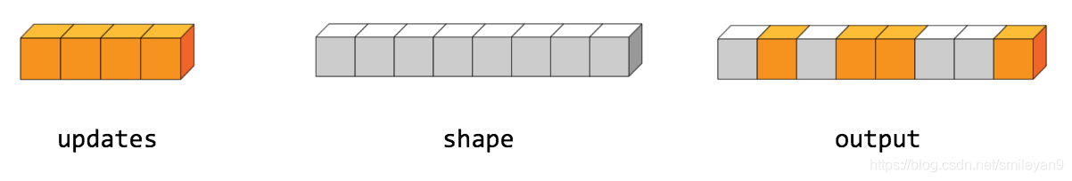
5.6.2 Update purposefully according to the coordinates tf.scatter_nd
tf.scatter_nd(indices, updates, shape) Purposefully update according to the coordinates .
example 1
As shown in the figure below , First specify shape Determines how the data is generated shape, In this case shape = 8, So the output data shape by 8,updates There are four in all , therefore indices You need to specify where to insert these three numbers , The index corresponding to the four numbers in the example is 4,3,1, 7 So when the placement is complete update The position corresponding to the number is 4 3 1 7.
import tensorflow as tf

indices = tf.constant([[4], [3], [1], [7]])
updates = tf.constant([9, 10, 11, 12])
shape = tf.constant([8])
scatter = tf.scatter_nd(indices, updates, shape)
print(scatter)
example 2
The understanding method is the same as above .
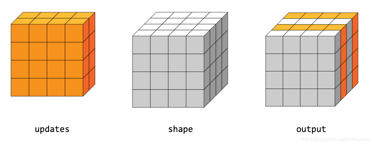
import tensorflow as tf

indices = tf.constant([[0], [2]])
updates = tf.constant([[[5, 5, 5, 5], [6, 6, 6, 6],
                        [7, 7, 7, 7], [8, 8, 8, 8]],
                       [[5, 5, 5, 5], [6, 6, 6, 6],
                        [7, 7, 7, 7], [8, 8, 8, 8]]])
shape = tf.constant([4, 4, 4])
scatter = tf.scatter_nd(indices, updates, shape)
print(scatter)
It's also easy to understand , It's just that the dimensions have increased and may look more complex .
The output content is :
[[[5, 5, 5, 5], [6, 6, 6, 6], [7, 7, 7, 7], [8, 8, 8, 8]],
 [[0, 0, 0, 0], [0, 0, 0, 0], [0, 0, 0, 0], [0, 0, 0, 0]],
 [[5, 5, 5, 5], [6, 6, 6, 6], [7, 7, 7, 7], [8, 8, 8, 8]],
 [[0, 0, 0, 0], [0, 0, 0, 0], [0, 0, 0, 0], [0, 0, 0, 0]]]
5.6.3 Generate coordinates tf.meshgrid
Take two-dimensional coordinates as an example , When specifying x The value set of , Appoint y The value set of , You can determine all (x, y) coordinate , The general idea is to double cycle .
but tf.meshgrid Provide a more efficient way , namely tf.meshgrid , As shown in the example :
import tensorflow as tf

x = [1, 2, 3]
y = [4, 5, 6]
X, Y = tf.meshgrid(x, y)

print(X)

print(Y)
The output content is :
tf.Tensor(
[[1 2 3]
 [1 2 3]
 [1 2 3]], shape=(3, 3), dtype=int32)
tf.Tensor(
[[4 4 4]
 [5 5 5]
 [6 6 6]], shape=(3, 3), dtype=int32)
Maybe it still doesn't look like coordinates , But just one Take... Respectively for one correspondence x and y that will do .
Consider using tf.stack Function generation is more like Coordinate tensor .
import tensorflow as tf

x = [1, 2, 3]
y = [4, 5, 6]
X, Y = tf.meshgrid(x, y)

tf.stack([X,Y],axis=2)
The output content is :
<tf.Tensor: shape=(3, 3, 2), dtype=int32, numpy=
array([[[1, 4],
        [2, 4],
        [3, 4]],

       [[1, 5],
        [2, 5],
        [3, 5]],

       [[1, 6],
        [2, 6],
        [3, 6]]], dtype=int32)>
6. Data loading
6.1 tf.keras.datasets
tf.keras.datasets The data set provided by the interface can be called textbook data set , All data sets come from the real environment , And it has been processed and can be well applied to model training and testing .
6.1.1 Data set Overview
So far (2020.10.29) until , The interface provides a total of 7 Data sets , The general introduction is as follows :
- Boston prices boston_housing : Provide some factors that may affect house prices and house prices , For regression tasks .
- Handwritten digit recognition mnist: Provide handwritten numeral recognition data set , Used to classify tasks .
- Clothing category identification fashion_mnist: Provide 10 Class picture , Include T T-shirt 、 A pair of jeans 、 Sandals, etc , Used to classify tasks .
- Item animal identification cifar10: Provide 10 Class picture , Include The plane 、 cat 、 Dogs, etc , Used to classify tasks .
- Item animal identification cifar100: Yes cifar10 Further subdivision , Each category is subdivided into 10 class , common 100 class , Used to classify tasks .
- Classification of film reviews imdb: Including film reviews and reviews , Used for two classification tasks 、 Text classification task .
- Classification of news topics reuters: Including news and topic classification , Used to classify tasks 、 Text classification task .
6.1.2 Loading method
The method of data loading is very simple , Just one line of code , With mnist For example :
import tensorflow as tf

(x_train, y_train),(x_test, y_test) = tf.keras.datasets.mnist.load_data()

print(x_train.shape)
print(y_train.shape)
print(x_test.shape)
print(y_test.shape)
The output content is :
(60000, 28, 28)
(60000,)
(10000, 28, 28)
(10000,)
The loading method of the other six datasets is similar , The only difference is tf.keras.datasets.mnist.load_data() Medium mnist .
If the dataset is loaded for the first time in your environment , It may take some time to download automatically , When downloading, the output content is roughly :
Downloading data from https://storage.googleapis.com/tensorflow/tf-keras-datasets/train-labels-idx1-ubyte.gz
32768/29515 [=================================] - 0s 10us/step
Downloading data from https://storage.googleapis.com/tensorflow/tf-keras-datasets/train-images-idx3-ubyte.gz
26427392/26421880 [==============================] - 13s 0us/step
Downloading data from https://storage.googleapis.com/tensorflow/tf-keras-datasets/t10k-labels-idx1-ubyte.gz
8192/5148 [===============================================] - 0s 0us/step
Downloading data from https://storage.googleapis.com/tensorflow/tf-keras-datasets/t10k-images-idx3-ubyte.gz
4423680/4422102 [==============================] - 4s 1us/step
(60000, 28, 28)
(60000,)
(10000, 28, 28)
(10000,)
The output content contains the download source of the dataset https://storage.googleapis.com/tensorflow/tf-keras-datasets/train-labels-idx1-ubyte.gz, So you can also consider copying the address and downloading it for other purposes , Of course , Certainly not as simple and convenient as the above method .
6.2 pandas Load data set
Use pandas When you encounter problems, you'd better check first pandas Official documents .
Only... Is mentioned here pandas load csv file , The loading method of files in other formats is similar .
6.2.1 Remote load
When using some public data sets , Use tf.keras.utils.get_file Remote loading of functions is more convenient , The use of functions is also very simple , After downloading, return to the absolute path of the downloaded file , Then load the data according to the absolute path .
So what we're talking about here Remote load intend “ Download to local , Load locally ”.
import pandas as pd
import tensorflow as tf

#  download  heart  Data sets
csv_file = tf.keras.utils.get_file('heart.csv', 'https://storage.googleapis.com/applied-dl/heart.csv')

#  Check the return value
print(csv_file)                        #  That is, the absolute path after downloading , for instance  '/home/yan/.keras/datasets/heart.csv'

#  Then use  pd.read_csv  that will do
df = pd.read_csv(csv_file)
df.head()
The output table is shown in the figure :

6.2.2 Local load
Local loading is easier , Everyone who has learned machine learning should have been exposed to pandas Local loading method .
import pandas as pd

csv_file = '/home/yan/.keras/datasets/heart.csv'
df = pd.read_csv(csv_file)
df.head()
6.2.3 format conversion
Because by default pandas Reading the file returns pandas.core.frame.DataFrame Format , Format conversion required .
import tensorflow as tf
import pandas as pd

csv_file = '/home/yan/.keras/datasets/heart.csv'
df = pd.read_csv(csv_file)
print(df.head())

#  Format this property  object  transformation  int
df['thal'] = pd.Categorical(df['thal'])
df['thal'] = df.thal.cat.codes

dataset = tf.data.Dataset.from_tensor_slices((df.values, target.values))
dataset
The output content is :
<TensorSliceDataset shapes: ((14,), ()), types: (tf.float64, tf.int64)>
6.3 load numpy Data sets
numpy Data sets are generally expressed in .npz Suffix a file , The loading method is also very simple , For example :
import numpy as np
import tensorflow as tf

DATA_URL = 'https://storage.googleapis.com/tensorflow/tf-keras-datasets/mnist.npz'

path = tf.keras.utils.get_file('mnist.npz', DATA_URL)
with np.load(path) as data:
    train_examples = data['x_train']
    train_labels = data['y_train']
    test_examples = data['x_test']
    test_labels = data['y_test']

train_dataset = tf.data.Dataset.from_tensor_slices((train_examples, train_labels))
test_dataset = tf.data.Dataset.from_tensor_slices((test_examples, test_labels))
6.4 Loading pictures
There are many differences between loading image data sets and those mentioned above , For example, image data must be multiple files , Instead of a single file that has been processed and merged , So you need some processing skills when loading , Even for large drawings, they need to be cut and loaded one by one .
Here's an example of a variety of flowers that Google provides download addresses picture .
6.4.1 Download the pictures
If the Internet speed is not good, it will take a few minutes , In general 1 It can be downloaded in minutes .
import tensorflow as tf

import pathlib
dataset_url = "https://storage.googleapis.com/download.tensorflow.org/example_images/flower_photos.tgz"
data_dir = tf.keras.utils.get_file(origin=dataset_url,
                                   fname='flower_photos',
                                   untar=True)
data_dir = pathlib.Path(data_dir)

data_dir
The output content is :
PosixPath('/home/yan/.keras/datasets/flower_photos')
You can check all the contents in this directory , It includes the following contents :
daisy/ dandelion/ LICENSE.txt roses/ sunflowers/ tulips/.
6.4.2 view picture
Check the data before preprocessing , Look at the flowers .
import tensorflow as tf
import PIL
import pathlib
dataset_url = "https://storage.googleapis.com/download.tensorflow.org/example_images/flower_photos.tgz"
data_dir = tf.keras.utils.get_file(origin=dataset_url,
                                   fname='flower_photos',
                                   untar=True)
data_dir = pathlib.Path(data_dir)

roses = list(data_dir.glob('roses/*'))
PIL.Image.open(str(roses[0]))

6.4.3 Use tf.keras.preprocessing Load data
The process is very simple , It should be noted that those parameters .
import tensorflow as tf
import pathlib
dataset_url = "https://storage.googleapis.com/download.tensorflow.org/example_images/flower_photos.tgz"
data_dir = tf.keras.utils.get_file(origin=dataset_url,
                                   fname='flower_photos',
                                   untar=True)
data_dir = pathlib.Path(data_dir)

batch_size = 32
img_height = 180
img_width = 180

train_ds = tf.keras.preprocessing.image_dataset_from_directory(
    data_dir,
    validation_split=0.2,
    subset="training",
    seed=123,
    image_size=(img_height, img_width),
    batch_size=batch_size)

val_ds = tf.keras.preprocessing.image_dataset_from_directory(
  data_dir,
  validation_split=0.2,
  subset="validation",
  seed=123,
  image_size=(img_height, img_width),
  batch_size=batch_size)

type(train_ds)
The output content is :
Found 3670 files belonging to 5 classes.
Using 2936 files for training.
Found 3670 files belonging to 5 classes.
Using 734 files for validation.
<BatchDataset shapes: ((None, 180, 180, 3), (None,)), types: (tf.float32, tf.int32)>
Here is just a simple example of loading pictures , For more training and testing of the model, please refer to Official documents
6.5 Load text
The method of loading text data is similar to that of pictures , Attention should be paid to the different parameters .
import tensorflow as tf
import pathlib
from tensorflow.keras import preprocessing

from tensorflow.keras import utils

data_url = 'https://storage.googleapis.com/download.tensorflow.org/data/stack_overflow_16k.tar.gz'

data_dir = tf.keras.utils.get_file(origin=dataset_url,
                                   fname='flower_photos',
                                   untar=True)
dataset = utils.get_file(
    'stack_overflow_16k.tar.gz',
    data_url,
    untar=True,
    cache_dir='stack_overflow',
    cache_subdir='')

train_dir = dataset_dir/'train'
# list(train_dir.iterdir())

dataset_dir = pathlib.Path(dataset).parent

batch_size = 32
seed = 42

raw_train_ds = preprocessing.text_dataset_from_directory(
    train_dir,
    batch_size=batch_size,
    validation_split=0.2,
    subset='training',
    seed=seed)

raw_val_ds = preprocessing.text_dataset_from_directory(
    train_dir,
    batch_size=batch_size,
    validation_split=0.2,
    subset='validation',
    seed=seed)

type(raw_train_ds)
The output content is :
Found 8000 files belonging to 4 classes.
Using 6400 files for training.
Found 8000 files belonging to 4 classes.
Using 1600 files for validation.
tensorflow.python.data.ops.dataset_ops.BatchDataset
7. summary
I sorted out my study notes , Unconsciously wrote so long ( According to the csdn Blog site statistics about 3 swastika ), In general, it's very simple tensorflow2 Basic knowledge of , I hope it can be written as a dictionary tool , Come here and have a look when you need it , If you can find it, review it , If you can't find it, update this blog .
Of course , Also hope to help others in use tensorflow2 People with similar problems , If you think there is something unclear or wrong , Please be sure to comment later , Be sure to watch and think carefully , thank !
Smileyan
2020.10.25 21.02 Release
2020.10.28 21:41 to update
版权声明
本文为[smile-yan]所创,转载请带上原文链接,感谢
https://yzsam.com/2022/04/202204210553132976.html
边栏推荐
- Sqoop imports tinyint type fields to boolean type
- Redis installation (centos7 command line installation)
- Investigate why close is required after sqlsession is used in mybatties
- NC basic usage 3
- R语言ggplot2可视化:ggplot2可视化散点图并使用geom_mark_ellipse函数在数据簇或数据分组的数据点周围添加椭圆进行注释
- 使用 WPAD/PAC 和 JScript在win11中进行远程代码执行
- 【目标跟踪】基于帧差法结合卡尔曼滤波实现行人姿态识别附matlab代码
- Alicloud: could not connect to SMTP host: SMTP 163.com, port: 25
- Computing the intersection of two planes in PCL point cloud processing (51)
- 论文写作 19: 会议论文与期刊论文的区别
猜你喜欢
Leetcode XOR operation
![[numerical prediction case] (3) LSTM time series electricity quantity prediction, with tensorflow complete code attached](/img/73/ba9fb872aa279405204c411c18f348.png)
[numerical prediction case] (3) LSTM time series electricity quantity prediction, with tensorflow complete code attached
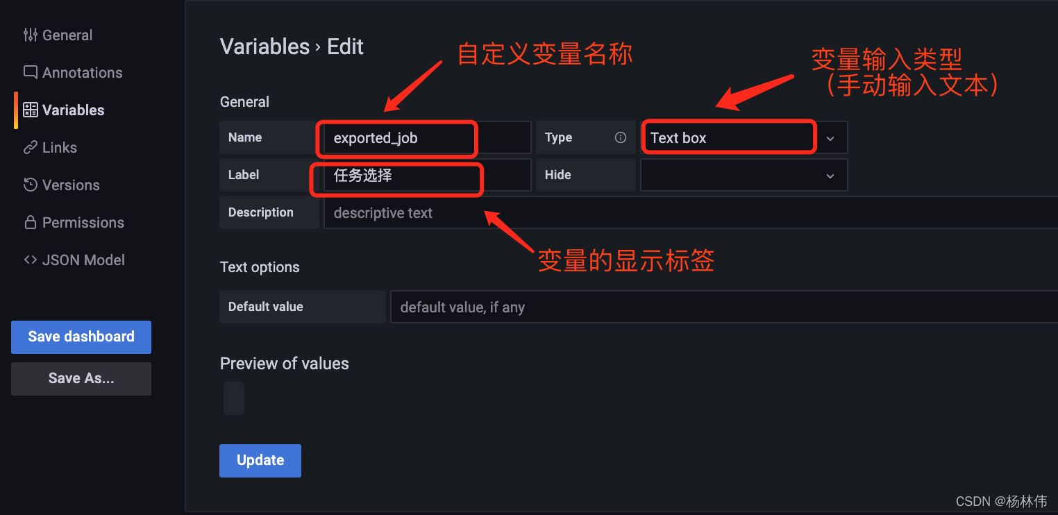
Grafana shares links with variable parameters
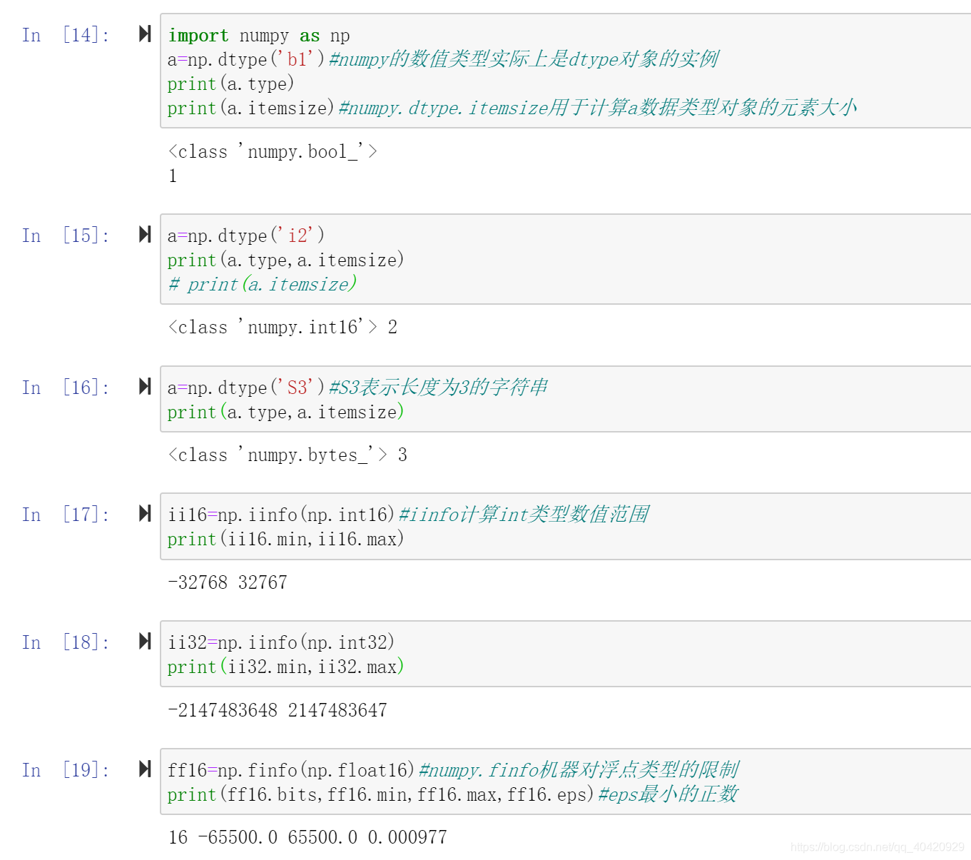
Numpy - creation of data type and array
Leetcode dynamic planning training camp (1-5 days)
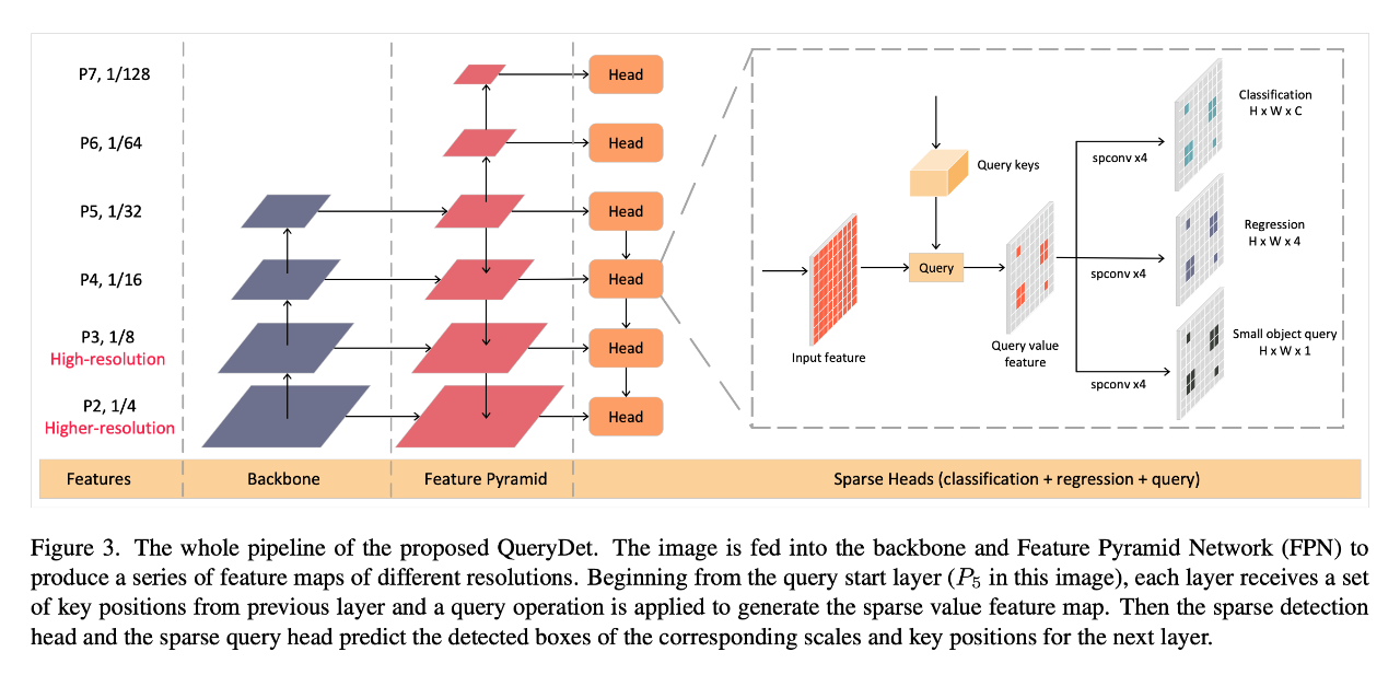
CVPR 2022 | querydet: use cascaded sparse query to accelerate small target detection under high resolution
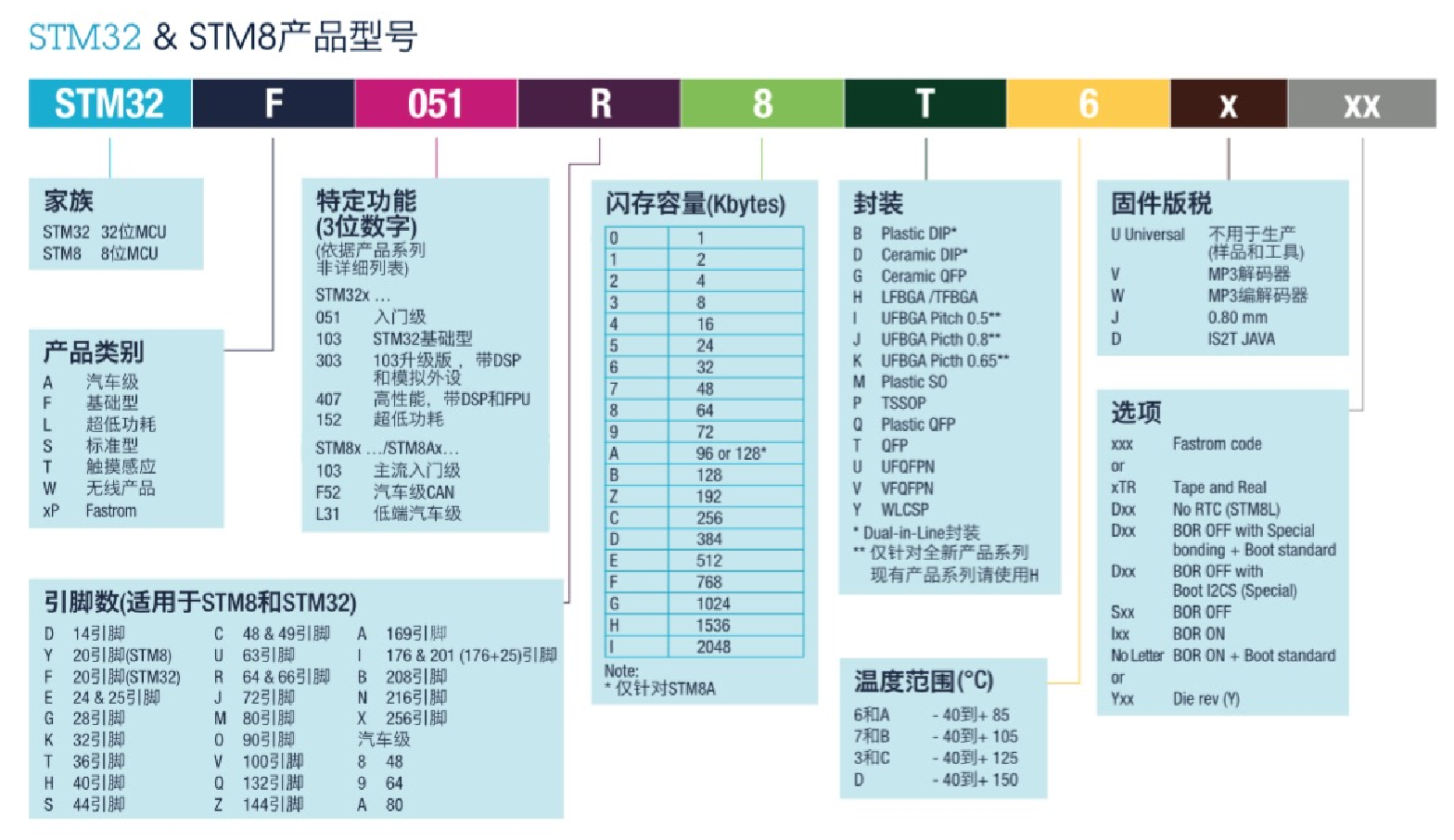
STM32基础知识

Error reported by Azkaban: Azkaban jobExecutor. utils. process. ProcessFailureException: Process exited with code 127
![Es error: request contains unrecognized parameter [ignore_throttled]](/img/17/9131c3eb023b94b3e06b0e1a56a461.png)
Es error: request contains unrecognized parameter [ignore_throttled]
考研英语唐叔的语法课笔记
随机推荐
selenium. common. exceptions. WebDriverException: Message: ‘chromedriver‘ executable needs to be in PAT
考研英语唐叔的语法课笔记
The textarea cursor cannot be controlled by the keyboard due to antd dropdown + modal + textarea
Paper writing 19: the difference between conference papers and journal papers
【2022】将3D目标检测看作序列预测-Point2Seq: Detecting 3D Objects as Sequences
Unity 模型整体更改材质
Unity general steps for creating a hyper realistic 3D scene
nc基础用法3
MySQL 进阶 锁 -- MySQL锁概述、MySQL锁的分类:全局锁(数据备份)、表级锁(表共享读锁、表独占写锁、元数据锁、意向锁)、行级锁(行锁、间隙锁、临键锁)
Cadence Orcad Capture CIS更换元器件之Link Database 功能介绍图文教程及视频演示
Handwritten Google's first generation distributed computing framework MapReduce
Vericrypt file hard disk encryption tutorial
Numpy Index & slice & iteration
How about CICC fortune? Is it safe to open an account
R语言survival包coxph函数构建cox回归模型、ggrisk包ggrisk函数和two_scatter函数可视化Cox回归的风险评分图、解读风险评分图、基于LIRI数据集(基因数据集)
JDBC tool class jdbcconutil gets the connection to the database
Is the wechat CICC wealth high-end zone safe? How to open an account for securities
Es index (document name) fuzzy query method (database name fuzzy query method)
CVPR 2022 | querydet: use cascaded sparse query to accelerate small target detection under high resolution
selenium.common.exceptions.WebDriverException: Message: ‘chromedriver‘ executable needs to be in PAT