当前位置:网站首页>Introduction and application of quantitative trading strategies
Introduction and application of quantitative trading strategies
2022-08-10 03:20:00 【Dark horse programmer official】
目录
一、Shares of quantitative strategy is introduced
三、Many factors strategy and theory of
1、What is the factor to choose a strategy more
7、About mining and how to do it
8、 案例:市值因子(Alpha因子)Choose a strategy
四、Many factors strategy process
1、 Many factors strategy process
2、 More certainty factor strategy
4、 About research platform for function
2、 What is the factor to deal with the extreme value
3、 Market neutralization treatment-回归法
5、 案例:Remove the price-to-book The contact between the value of part
一、Shares of quantitative strategy is introduced
Stock there are two kinds of quantitative trading strategy is the most basic form,趋势交易(技术分析)And market neutral(基本面分析),Commonly used method forMany factors to pick stocks and track trends
注:Whether the trend tracking strategy or multiple factor to choose a strategy,Are in order to obtain certain excess returns.Trend tracking means to get through a variety of trading strategy,While many factor to choose a strategy of the stock is through stock selection
收益到底从何而来?What affect stock returns?
二、Alpha和Beta
Each investment strategy yields can be decomposed into two parts:
- Part related to the market completely,The average yield of the entire market multiplied by a beta.Beta can be called the portfolio risk of system
- The other part has nothing to do with the market called alpha(Alpha)

1、Alpha很难得,Beta很容易.
2、AlphaIs the selectivity,跑赢市场.
3、BetaJust have a market to keep up with,When risky escape
三、Many factors strategy and theory of
1、What is the factor to choose a strategy more
Many factor to choose a strategy is a kind of application is very extensive stock selection strategy,The basic idea is to find some and yields the most relevant factor.
2、 多因子(Alpha因子)的种类
- According to the factor analysis point of view

- 1、基本面因子
- 价值因子
- 盈利因子
- 成长因子
- Capital structure factor
- Operational factors
- Liquidity factor
- 2、技术因子
- 动量因子
- 趋势因子
- 市值因子
- 波动因子
- Volume factor
- According to the factor source's point of view

- 公司层面
- 价值因子
- 成长因子
- 规模因子
- 等
- 市场层面
- 趋势因子
- 动量因子
- 市值因子
- 外部环境层面
- 宏观环境
- 行业环境
Categories of factors subdivision


The advantage of multiple factor strategy
- Multiple factor,The source of the alpha gains rich,Many factors steady
- According to the change of market environment to select the optimal factor and weight,Model can be modified
Many factors strategy theory source of?(重要)What influence the yield of stock?
3、 资产定价模型(CAPM)

- ri:The yield of securities
- rF:无风险利率
- rM:市场收益率
- rM-rF: 风险溢价
- β: The correlation of a company and the market
This model can be understood as a single factor model-系统风险,We only go with the market.
4、套利定价理论(APT模型)
Assuming that securities with a group of unknown factor(特征)线性相关

APTModel is equivalent to more than one factor model,Stock returns is obtained by weighting coefficient regression.But there is no point out the specific factor(特征)是什么
5、 FF三因子模型
Fama和French 1992年对美国股票市场决定不同股票回报率差异的因素的研究发现(Find value smaller、Book with low value of two types of companies are more likely to achieve better than market average return),Excess returns can be made of it to the three factors to explain.市场资产组合、市值因子(SMB)、账面市值比因子(HML).

Three factor model is pointed out that the scale factor、价值因子.
Find value smaller、Book with low value of two types of companies are more likely to achieve better than market average return
Means the value of portfolio of smaller companies,Can be expected to bring higher returns,With a higher risk.所以在2017Years ago, within a period of time,Most quantitative company in the market value of small target screening can get very high returns
在过去20年里面,Many scholars on the three factor model for empirical analysis,Find some stockalpha显著不为0,This shows that three of the three factor model risk(因素)Does not explain all the excess returns.
6、 FF五因子模型
Fama和FrenchFound outside the risk,And profitability risk、Investment risk also can bring the excess returns of stocks,并于2015Put forward the five factor model

Five factor model is actually increased the profit factor and growth factor these two kinds of factor
Similar to three factors,Parameter estimation method is still using multiple linear regression method,这里的a_iIs the five factor model which has yet to explain the excess return of.
7、About mining and how to do it


A lot of data, or securities firms report,There are a lot of some of the new method can be to explore
8、 案例:市值因子(Alpha因子)Choose a strategy
8.1 结果

8.2 To select values from the market value of small stock
- Selected financial data screening
- For daily warehouse(The warehouse cycle frequency factor picking stocks will be smaller)
8.3 代码
def init(context):
    context.limit = 20


def before_trading(context):
    # Access to financial data of the market value,Then according to the value of order
    fund = get_fundamentals(
        query(
            fundamentals.eod_derivative_indicator.market_cap
        ).order_by(
            fundamentals.eod_derivative_indicator.market_cap.asc()
        ).limit(
            context.limit
        )
    )

    # 将这20Stock code
    context.stocks = fund.columns


def handle_bar(context, bar_dict):
    # First draw a portfolio of positions do you have any stock,Note the position here even as0,但是
    # Stock name also in
    holding = []

    for stock in context.portfolio.positions.keys():

        # Judge whether the current stock holdings
        if context.portfolio.positions[stock].quantity > 0:
            holding.append(stock)

    # Determine which to sell,What to buy
    to_sell = set(holding) - set(context.stocks)
    to_buy = context.stocks

    # Buy and sell judgment
    for sell in to_sell:
        order_target_percent(sell, 0)

    # The proportion of purchase
    percent = 1.0 / len(to_buy)

    for buy in to_buy:
        order_target_percent(buy, percent)
四、Many factors strategy process
1、 Many factors strategy process

Focused on the exploration and processing factors
We can draw the following steps
- 因子挖掘
- Factor data processing
- 去极值
- 标准化
- 中性化
- The effectiveness of the single factor test
- 因子IC分析
- Factor of yield analysis
- Factor in the direction of the
- Multiple factor correlation and composite analysis
- Correlation factor
- Factor synthesis
- Factor data processing
- 回测
- More weight factor to pick stocks
- The warehouse cycle
2、 More certainty factor strategy
- 1、Choose which the direction of the factor and factor determine
- 2、因子的权重(Scoring method and regression method)
- 3、The warehouse cycle
其中1Step part of the exploration and processing of the factor,2和3Step is chosen factor to measure parts
3、Factor to dig what to do?

Because this part is not to measure,So we need in a separate study platform using a specific interface analysis.RQPlatform provides such a research platform for us to dig factor
4、 About research platform for function
On the study of the factors when we need to get more range of history data to study,So the function of platform will is not the same as back into test
About research platform document:https://www.ricequant.com/api/research/chn
4.1get_price - To obtain contracts historical data
get_price(order_book_id, start_date='2013-01-04', end_date='2014-01-04', frequency='1d', fields=None, adjust_type='pre', skip_suspended =False, country='cn')To obtain a list specified contracts or contracts the historical data of(Contains the commencement date,In minutes line or).Currently only support China market.At the time of writing strategies is recommended to usehistory_bars
参数
| 参数 | 类型 | 说明 |
|---|---|---|
| order_book_id | str OR str list | 合约代码,可传入order_book_id, order_book_id list |
| start_date | str, datetime.date, datetime.datetime, pandasTimestamp | 开始日期,默认为'2013-01-04'.When using trading,用户必须指定 |
| end_date | str, datetime.date, datetime.datetime, pandasTimestamp | 结束日期,默认为'2014-01-04'.When using trading,The day before the default strategy for the current date |
| frequency | str | 历史数据的频率. Now support/The historical data of minute level,默认为'1d'.Users are free to choose different frequency,例如'5m'代表5分钟线 |
| fields | str OR str list | 返回字段名称 |
| adjust_type | str | 前复权处理.前复权 - pre,后复权 - post,不复权 - none,Back to the measurement using - internal需要注意,internalConsistent data and used to test,Just break up events to the answer authority before the price and volume,Does not take into account dividends for the impact of stock price.So before and after the share out bonus,The price will jump in. |
| skip_suspended | bool | Whether or not to skip the suspension data.默认为False,不跳过,With suspended before filling the data.TrueIs to skip the suspension period.注意,当设置为True时,函数order_book_idOnly supports a single contract to |
| country | str | The default is the Chinese market('cn'),Currently only support China market |
返回
- 传入一个order_book_id,多个fields,函数会返回pandas DataFrame
- 传入一个order_book_id,一个field,函数会返回pandas Series
- 传入多个order_book_id,一个field,函数会返回pandas DataFrame
- 传入多个order_book_id,函数会返回pandas Panel
案例:
- To obtain a historical date line stock market(返回pandas DataFrame):
[In]get_price('000001.XSHE', start_date='2015-04-01', end_date='2015-04-12')
[Out]
open    close    high    low    total_turnover    volume    limit_up    limit_down
2015-04-01    10.7300    10.8249    10.9470    10.5469    2.608977e+09    236637563.0    11.7542    9.6177
2015-04-02    10.9131    10.7164    10.9470    10.5943    2.222671e+09    202440588.0    11.9102    9.7397
2015-04-03    10.6486    10.7503    10.8114    10.5876    2.262844e+09    206631550.0    11.7881    9.6448
2015-04-07    10.9538    11.4015    11.5032    10.9538    4.898119e+09    426308008.0    11.8288    9.6787
2015-04-08    11.4829    12.1543    12.2628    11.2929    5.784459e+09    485517069.0    12.5409    10.2620
2015-04-09    12.1747    12.2086    12.9208    12.0255    5.794632e+09    456921108.0    13.3684    10.9403
2015-04-10 12.2086 13.4294 13.4294 12.1069 6.339649e+09 480990210.0 13.4294 10.9877- Get the stock list history the daily closing price(返回pandas DataFrame):
[In]get_price(['000024.XSHE', '000001.XSHE', '000002.XSHE'], start_date='2015-04-01', end_date='2015-04-12', fields='close')
[Out]
000024.XSHE    000001.XSHE    000002.XSHE
2015-04-01    32.1251    10.8249    12.7398
2015-04-02    31.6400    10.7164    12.6191
2015-04-03    31.6400    10.7503    12.4891
2015-04-07    31.6400    11.4015    12.7398
2015-04-08    31.6400    12.1543    12.8327``
2015-04-09    31.6400    12.2086    13.5941
2015-04-10 31.6400 13.4294 13.2969- Get the stock list history date line co(返回pandas DataPanel):
[In]get_price(['000024.XSHE', '000001.XSHE', '000002.XSHE'], start_date='2015-04-01', end_date='2015-04-12')
[Out]
<class 'rqcommons.pandas_patch.HybridDataPanel'>
Dimensions: 8 (items) x 7 (major_axis) x 3 (minor_axis)
Items axis: open to limit_down
Major_axis axis: 2015-04-01 00:00:00 to 2015-04-10 00:00:00
Minor_axis axis: 000024.XSHE to 000002.XSHE
4.2 get_trading_dates - 获取交易日列表
get_trading_dates(start_date, end_date, country='cn')To obtain a list of one country market trading day(Commencement date to judge).Currently only support China market.
参数
| 参数 | 类型 | 说明 |
|---|---|---|
| start_date | str, datetime.date, datetime.datetime, pandasTimestamp | 开始日期 |
| end_date | str, datetime.date, datetime.datetime, pandasTimestamp | 结束日期 |
| country | str | The default is the Chinese market('cn'),Currently only support China market |
返回
datetime.date list - Transaction date list(除去周末、节假日)
范例
[In]get_trading_dates(start_date='20160505', end_date='20160505')
[Out]
[datetime.date(2016, 5, 5)]
4.3 get_fundamentals - Query financial data
get_fundamentals(query, entry_date, interval=None, report_quarter=False)Access to historical financial data table.Currently support the Chinese market more than400个指标,具体请参考 Financial data document .Currently only support China market.We specifically for this function is optimized,Read the operation of the memory can greatly improve data acquisition speed. 注意:
- 使用get_fundamentals()Query financial data,We are all the release date of the annual report(announcement date)为准,Because only after the earnings release become open access to data on the market.Such as a company in the third quarter results in11月10号发布,As if from the query date for10月5号,That is earlier than the release date,Then the return is in the second quarter earnings data.
- For a fixed period of financial data, please useget_financials().
参数
| 参数 | 类型 | 说明 |
|---|---|---|
| query | SQLAlchemyQueryObject | SQLAlchmey的Query对象.Which can be in'query'Fill in need within the query index,'filter'Fill in the data filtering conditions.具体可参考 sqlalchemy's query documentation Learn to use more convenient query.From the perspective of a data scientist,sqlalchemy的使用比sqlMore simple and powerful |
| entry_date | str, datetime.date, datetime.datetime, pandasTimestamp | Financial data query baseline start date |
| interval | str | Query the interval of financial data.例如,填写'5y',则代表从entry_date开始(包括entry_date)回溯5年,Returns the time data for years interval.'d' - 天,'m' - 月(30天), 'q' - 季(90天),'y' - 年(365天) |
| report_quarter | bool | Is displayed during the reporting period,默认为False,不显示.'Q1' - 一季报,'Q2' - 半年报,'Q3' - 三季报,'Q4' - 年报 |
返回
pandas DataPanel - Financial data query result.
范例
fundamentals是一个重要的对象,Including the stock index table(eod_derivative_indicator),财务指标表(financial_indicator),利润表(income_statement),资产负债表(balance_sheet),现金流量表(cash_flow_statement)As well as the stock list(stock_code)等内容.结合SQLAlchemy的查找方式,To meet the demand of the user a variety of.
- Get some stock2015年1月10日及以前5年的营业收入(revenue)As well as operating cost(cost_of_good_sold)
[In]dp = get_fundamentals(query(fundamentals.income_statement.revenue, fundamentals.income_statement.cost_of_goods_sold
).filter(fundamentals.income_statement.stockcode.in_(['002478.XSHE', '000151.XSHE'])), '2015-01-10', '5y')

[In]dp
[Out]
<class 'pandas.core.panel.Panel'>
Dimensions: 2 (items) x 5 (major_axis) x 2 (minor_axis)
Items axis: revenue to cost_of_goods_sold
Major_axis axis: 2015-01-09 to 2011-01-10
Minor_axis axis: 002478.XSHE to 000151.XSHE

[In]dp['revenue']
[Out]
            002478.XSHE        000151.XSHE
2015-01-09    2.937843e+09    1.733703e+09
2014-01-10    2.926316e+09    8.839355e+08
2013-01-10    2.616532e+09    9.488980e+08
2012-01-10    2.681016e+09    6.205934e+08
2011-01-10    2.034147e+09    4.998120e+08
五、因子数据处理-去极值
学习目标
- 目标
- Show panel data、Difference between sequence data and section data of
- Know that processing factor data of each factor to the cross section of the data processing
- Understand the role of quantile
- Quantile to extreme value is applied to implement to extreme value quantile
- Understand the median absolute deviation method
- Implement the median absolute deviation method to extremum
- 了解3倍sigma法则
- 实现3倍sigmaMethod to extremum
- Comparison of three go to extreme value methods advantages and disadvantages of
- 应用
- 无
So in many factors of strategy,We analysis the factor of data is how to?Factor with the analysis of the yield,What should be the structure to provide?
1、 因子Panel结构分析

PandasThe panel of数据结构Is to store the three dimensional structure.Consists of cross section data and sequence data
1.1 截面数据
横截面数据:在同一时间,不同统计单位相同统计指标组成的数据列

1.2 序列数据
序列数据:Data collected at different time points,这类数据反映了某一事物、现象等随时间的变化状态或程度

Multiple factor analysis using cross-section data!!!
2、 What is the factor to deal with the extreme value
去极值并不是删除”异常数据”,而是将这些数据”拉回”到正常的值
注:Extremum can understand outliers or abnormal data
2.1 三种方法
- 分位数去极值
- 中位数绝对偏差去极值
- 正态分布去极值
When in contact with some statistical indicators before,Know the minimum most、平均值、方差、标准差等等.So here we use a call quantile indicators for go to extreme value
3、分位数去极值
So what is to extreme value quantile?Here we introduce several related concepts
- 1、中位数
- 2、四分位数
- 3、百分位数
3.1 中位数
定义:The median is the data in order of size,形成一个数列,The data in the sequence of the middle.中位数用Me(Median简写)表示
14、15、16、16、17、18、18、19、19、20、2l、11、22、22、23、24、24、25、26
中位数为:20,If there is no one in the middle of the number of,So in the middle of the two Numbers mean
Why need the median this index
There are four such as now,A年收入12万,B年收入10万,C年收入9万,D年收入10亿.Then we go to ask the average income for four,So everyone income $,明显不准确.So suppose we to find the median response their average income,先从小到大排列,9,10,12,10亿,So take the median,10+12/2 = 11万,This result to reflect all the average level of.So sometimes many areas in statistical average salaries,To feel the average,The result is not ideal because average.3.2 四分位数
即把所有数值由小到大排列并分成四等份,处于三个分割点位置的数值就是四分位数

- 第一四分位数 (Q1),又称“较小四分位数”,等于该样本中所有数值由小到大排列后第25%的数字.
- 第二四分位数 (Q2),又称“中位数”,等于该样本中所有数值由小到大排列后第50%的数字.
- 第三四分位数 (Q3),又称“较大四分位数”,等于该样本中所有数值由小到大排列后第75%的数字.
Have a quartile calculation case:http://wiki.mbalib.com/wiki/%E5%9B%9B%E5%88%86%E4%BD%8D%E6%95%B0
3.3 百分位数
In front of the median,Quartile are some special case.Percentile is the location data for whole a%位数.There are two kinds of the percentile call,quantile和percentile.他们之间的关系如下
0 quantile = 0 percentile
0.25 quantile = 25 percentile
0.5 quantile = 50 percentile
0.75 quantile = 75 percentile
1 quantile = 100 percentile
3.4 分位数去极值
3.4.1 原理
将指定分位数区间以外的极值用分位点的值替换掉
3.4.2 API
- from scipy.stats.mstats import winsorize
- scipy.stats.mstats.winsorize(a, limits=None)
- Returns a Winsorized version of the input array Parameters:
- a : sequence Input array.
- limits : float At the ends of the datapercentile的值
- Returns a Winsorized version of the input array Parameters:
3.5 案例:对pe_ratio进行去极值
3.5.1 Results the phenomenon of

3.5.2 分析
- Access to specify a date or range ofpe_ratioThe cross section data(The date of the interval period of data needs to be joining together)
- 分位数去极值
- Results compared with the results before going to extremum extremum to
3.5.3 代码
# Access to finance must fill in the date
factor = get_fundamentals(query(fundamentals.eod_derivative_indicator.pe_ratio), entry_date="20180103")[:, 0, :]

factor['pe_ratio'][:1000].plot()

# Percentile to extreme value
# 将2.5%Below the quantile values,替换
# 将97.5%The value of quantile above,替换
factor['pe_ratio1'] = winsorize(factor['pe_ratio'], limits=0.025)

factor['pe_ratio'][:1000].plot()
factor['pe_ratio1'][:1000].plot()
3.6 自实现分位数去极值
# The value of two quantile point
def quantile(factor,up,down):
 """分位数去极值  """
  up_scale = np.percentile(factor, up)
  down_scale = np.percentile(factor, down)
  factor = np.where(factor > up_scale, up_scale, factor)
  factor = np.where(factor < down_scale, down_scale, factor)
  return factor
4、中位数绝对偏差去极值
MADAlso known as the median absolute deviation method(Median Absolute Deviation),MAD 是一种先需计算所有因子与中位数之间的距离总和来检测离群值的方法.
4.1 计算方法
- 1、找出因子的中位数 median
- 2、得到每个因子值与中位数的绝对偏差值 |x – median|
- 3、得到绝对偏差值的中位数, MAD,median(|x – median|)
- 4、计算MAD_e = 1.4826*MAD,然后确定参数 n,做出调整
Remove the extremum judgment:

注:Usually the deviation from the median three timesMAD_e,If the sample meet normal distribution,且数据量较大,Can prove that the above data as outliers.The mean and standard deviation method than,中位数和MADThe calculation is not affected by abnormal extreme value,结果更加稳健.
4.2 Implement the median absolute deviation method
def mad(factor):
  """3倍中位数去极值
  """
  # 求出因子值的中位数
  med = np.median(factor)

  # 求出因子值与中位数的差值,进行绝对值
  mad = np.median(abs(factor - med))

  # 定义几倍的中位数上下限
  high = med + (3 * 1.4826 * mad)
  low = med - (3 * 1.4826 * mad)

  # 替换上下限以外的值
  factor = np.where(factor > high, high, factor)
  factor = np.where(factor < low, low, factor)
  return factor
4.3案例:对pe_ratio进行去极值
4.3.1 结果

4.3.2 分析
- 中位数绝对偏差去极值
- Results compared with the results before going to extremum extremum to
4.3.3 代码
# For the median to extreme value
factor['pe_ratio2'] = mad(factor['pe_ratio'])
# 显示
factor['pe_ratio'][:500].plot(color='g')
factor['pe_ratio2'][:500].plot(color='r')
5、正态分布去极值
3sigma原则

5.1 3sigma方法实现
# 3sigma原则
def three_sigma(factor):

  # The mean and standard deviation of factor data
  mean = factor.mean()
  std = factor.std()
  # About data and subtract3个标准差
  high = mean + (0.01 * std)
  low = mean - (0.01 * std)

  # Replace the extreme data
  factor = np.where(factor > high, high, factor)
  factor = np.where(factor < low, low, factor)

  return factor
5.2 案例:对pe_ratio进行去极值
5.2.1 结果

5.2.2 分析
- 3sigmaMethods to extreme value
- Results compared with the results before going to extremum extremum to
5.2.3 代码
# For the median to extreme value
factor['pe_ratio3'] = three_sigma(factor['pe_ratio'])

factor['pe_ratio'][:500].plot(color='g')
factor['pe_ratio3'][:500].plot(color='r')
六、因子数据处理-标准化
1、对pe_ratio标准化
from sklearn.preprocessing import StandardScaler
std = StandardScaler()
std.fit_transform(factor['pe_ratio2'])
2、实现标准化
在调用fit_transform之后,The type of data will becomearray数组.Don't modify the original type,我们可以简单的实现
def stand(factor):
  """自实现标准化
  """
  mean = factor.mean()
  std = factor.std()
  return (factor - mean)/std
调用
factor['pb_ratio'] = stand(factor['pb_ratio'])七、因子数据处理-市值中性化
1、 为什么需要中性化处理?什么时候用?
Market value neutralization to inFactor to pick stocks back to the time of measurement(Do not belong to the factor used when mining)防止选到的股票集中在固定的某些股票当中.
怎么理解?
1.1 市值影响
默认大部分因子当中都包含了市值的影响,所以当我们通过一些指标选择股票的时候,每个因子都会提供市值的因素,Yes choose stock more concentrated,也就是选股的标准不太好.
比如:市净率会与市值有很高的相关性,这时如果我们使用未进行市值中性化的市净率,选股的结果会比较集中.
2、怎么去除市值影响
Before we combine algorithm or knowledge,The method can remove a factor influence on another factor?

3、 Market neutralization treatment-回归法
In each time section on the use of all stock data in cross-section regression equation,x为市值因子,yTo remove the value influence factor

通过拟合找到x,y的关系公式,预测的时候会出现偏差?这个偏差是什么?
This deviation is retained a factor to remove the influence of market value part
4、回归法API
- from sklearn.linear_model import LinearRegression
- 把市值设置成特征,市值不进行任何处理
- Set the other factors as the target
5、 案例:Remove the price-to-book The contact between the value of part
5.1 分析
- 获取两个因子数据
- 对目标值因子-市净率进行去极值、标准化处理
- 建立市值与市净率回归方程
- 通过回归系数,预测新的因子结果y_predict
- 求出市净率与y_predict的偏差即为新的因子值
5.2 代码
# 1、获取这两个因子数据
q = query(fundamentals.eod_derivative_indicator.pb_ratio,
         fundamentals.eod_derivative_indicator.market_cap)

# 获取的是某一天的横截面数据
factor = get_fundamentals(q, entry_date="2018-01-03")[:, 0, :]

# 先对pb_ratio进行去极值标准化处理
factor['pb_ratio'] = mad(factor['pb_ratio'])
factor['pb_ratio'] = stand(factor['pb_ratio'])

# 确定回归的数据
# x:市值
# y : 因子数据
x = factor['market_cap'].reshape(-1, 1)
y = factor['pb_ratio']

# 建立回归方程并预测
lr = LinearRegression()
lr.fit(x, y)
y_predict = lr.predict(x)

# 去除线性的关系,留下误差作为该因子的值
factor['pb_ratio'] = y - y_predict边栏推荐
猜你喜欢

In automated testing, test data is separated from scripts and parameterized methods

微透镜阵列后光传播的研究

Deep Learning (5) CNN Convolutional Neural Network

2022 Top Net Cup Quals Reverse Partial writeup
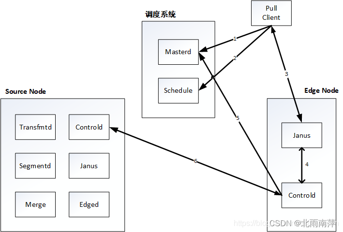
Janus actual production case

Fusion Compute网络虚拟化

OpenCV图像处理学习三,Mat对象构造函数与常用方法

组件的使用

Initial attempt at UI traversal
月薪35K,靠八股文就能做到的事,你居然不知道
随机推荐
Janus实际生产案例
[Swoole Series 3.5] Process Pool and Process Manager
OpenCV图像处理学习一,加载显示修改保存图像相关函数
2022.8.8考试摄像师老马(photographer)题解
C# winform 单选框
【QT】QT项目:自制Wireshark
元素的盒子模型+标签的尺寸大小和偏移量+获取页面滚动距离
《GB39707-2020》PDF download
【二叉树-困难】124. 二叉树中的最大路径和
mysql -sql编程
【二叉树-中等】687. 最长同值路径
官宣出自己的博客啦
MySQL:你做过哪些MySQL的优化?
In automated testing, test data is separated from scripts and parameterized methods
sqlmap dolog外带数据
2022.8.8考试游记总结
T5:Text-toText Transfer Transformer
算法与语音对话方向面试题库
C# 正则表达式分组查询
Fusion Compute网络虚拟化